Design of Experiments (Active Learning) with Bayesian Optimization
Contents
Note
This lecture is going to:
introduce the concepts of active learning or design of experiments
discuss the tradeoffs between exploration and exploitation
show several baseline exploration strategies
random sampling
latin hypercube sampling
sobol sampling
show how one open source package (scikit-optimize) uses sklearn GP regressors to implement this
demonstrate this for a physical experiment by optimizing paper helicopters using sigopt!
Design of Experiments (Active Learning) with Bayesian Optimization#
Design of Experiments (DoE), or active learning, is the research area of choosing which parameters to sample to learn about or optimize some system (usually an experiment or expensive simulation).
A few common use cases:
We want to maximize/minimize some metric
Tune elemental composition to optimize some property
Fine the best temperature to operate some process
Build a surrogate (fast) model for some experimental process
Develop a ML model that can reproduce the output of a large chemical plant
We will repeatedly sample a process and use that information to select new points to sample. We will try to accomplish some goal with the minimum number of evaluations. There are many strategies that we can use.
Trial Function#
As a trial function, let’s try to find the highest value of the function
where \(\epsilon\) is random noise with a scale of 0.1. We’ll limit ourselves to the region \(x\in[0,1]\).
Let’s define and plot the objective function first!
import numpy as np
import plotly.express as px
def objective(x, noise=0.05):
noise = np.random.normal(loc=0, scale=noise, size=x.shape)
return (x**2 * np.sin(5 * np.pi * x) ** 6.0) + noise
# Plot the objective function evaluated at 100 evenly spaced points
x_eval = np.linspace(0, 1, 100)
fig = px.scatter(x=x_eval, y=objective(x_eval))
# Add a line for the actual function evaluation!
x_eval = np.linspace(0, 1, 1000)
fig.add_scatter(x=x_eval, y=objective(x_eval, noise=0))
There are five local maxima in this range. The noise is significant here. The best maxima is the one to the right. We got this by doing 100 function evaluations.
Uniform or random sampling strategies#
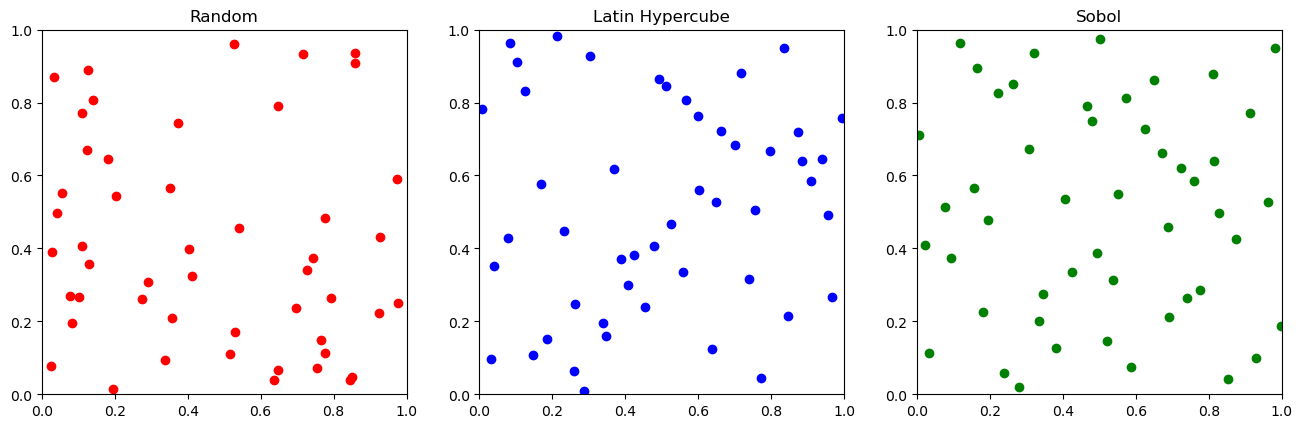
If we don’t want to build a model or do local optimizations, we can try to optimize a function \(f(x,y)\) by randomly sampling with various parameters. Three of the most common strategies are:
random sampling: Just pick random parameters and try them
latin hypercube sampling: try to pick points to improve the variability of the outputs
Sobol sampling: try to pick random points with the goal of equally covering the entire space and then going back and filling in the space
These are pretty simple, but usually helpful for selecting the first points to try. A rough rule of thumb is to sample ~5-10 or ~2D (where D is the number of dimensions) points before trying to use a fancy ML based method if you don’t know anything about the system. Let’s visualize the strategies in two dimensions!
import numpy as np
from scipy.stats import qmc
N = 50
# Generate N random samples in two dimensions
random_samples = np.random.uniform(0, 1, size=(N, 2))
# Generate N latin hypercube samples
latin_hypercube_samples = qmc.LatinHypercube(2).random(N)
# Generate N sobol samples in two dimensions
sobol_samples = qmc.Sobol(d=2, scramble=True).random(N)
/tmp/ipykernel_1256/2070957824.py:13: UserWarning:
The balance properties of Sobol' points require n to be a power of 2.
Now let’s make a little animation to see how the differenget
# Make a matplotlib animation!
import matplotlib.pyplot as plt
import numpy as np
from matplotlib import animation, rc
# Make the plots
fig, ax = plt.subplots(ncols=3, nrows=1, figsize=(16, 9))
(pt_random,) = ax[0].plot([], [], "ro")
(pt_latin_hypercube,) = ax[1].plot([], [], "bo")
(pt_sobol,) = ax[2].plot([], [], "go")
ax[0].set_xlim(0, 1)
ax[0].set_ylim(0, 1)
ax[0].set_adjustable("box")
ax[0].set_aspect("equal")
ax[0].set_title("Random")
ax[1].set_xlim(0, 1)
ax[1].set_ylim(0, 1)
ax[1].set_aspect("equal")
ax[1].set_adjustable("box")
ax[1].set_title("Latin Hypercube")
ax[2].set_xlim(0, 1)
ax[2].set_ylim(0, 1)
ax[2].set_aspect("equal")
ax[2].set_adjustable("box")
ax[2].set_title("Sobol")
# Initialize and clear the data!
def init():
pt_random.set_data([], [])
pt_latin_hypercube.set_data([], [])
pt_sobol.set_data([], [])
return (pt_random, pt_latin_hypercube, pt_sobol)
def animate(i):
# Set the data for a given frame
pt_random.set_data(random_samples[:i, 0], random_samples[:i, 1])
pt_latin_hypercube.set_data(
latin_hypercube_samples[:i, 0], latin_hypercube_samples[:i, 1]
)
pt_sobol.set_data(sobol_samples[:i, 0], sobol_samples[:i, 1])
return (pt_random, pt_latin_hypercube, pt_sobol)
# Make the animation!
anim = animation.FuncAnimation(
fig,
animate,
init_func=init,
frames=N,
interval=1000,
repeat_delay=5000,
blit=True,
)
rc("animation", html="jshtml")
anim
Evaluation of simple sampling strategies on optimizing the test function#
Let’s see how these three strategies work for sampling the test function above.
Base case: random sampling#
The easiest thing we can do is randomly pick points in the range. For a given number of random samples, we can evaluate all of them and see what the best is!
import pandas as pd
# Make an empty dataframe!
df_random = pd.DataFrame()
num_samples = list(range(1, 100))
for n in num_samples:
# Run 10 trials with n samples!
y = [np.max(objective(np.random.uniform(0, 1, size=(n,)))) for i in range(100)]
# Add the results to the dataframe
df_random = pd.concat(
(
df_random,
pd.DataFrame(
{"num_samples": [n], "objective": [np.mean(y)], "stdev": [np.std(y)]}
),
),
ignore_index=True,
)
# Plot with error bars!
px.line(df_random, x="num_samples", y="objective", error_y="stdev")
Note that our process - pick the best value of the random points is actually not giving us quite the right answer when we evaluate many times, since we also have a bit of noise in the measurements!
We can see that to get close to the real value of ~0.80 we need ~80 function evaluations. At 20 evaluations our best value is ~0.65.
Latin hypercube sampling#
import pandas as pd
import plotly.graph_objects as go
from scipy.stats import qmc
# Make an empty dataframe!
df_latinhypercube = pd.DataFrame()
num_samples = list(range(1, 100))
for n in num_samples:
# Run 10 trials with n samples!
y = [np.max(objective(qmc.LatinHypercube(2).random(n))) for i in range(100)]
# Add the results to the dataframe
df_latinhypercube = pd.concat(
(
df_latinhypercube,
pd.DataFrame(
{"num_samples": [n], "objective": [np.mean(y)], "stdev": [np.std(y)]}
),
),
ignore_index=True,
)
fig = go.Figure()
fig.add_scatter(
x=df_random["num_samples"],
y=df_random["objective"],
error_y={"array": df_random["stdev"]},
name="Random sampling",
)
fig.add_scatter(
x=df_latinhypercube["num_samples"],
y=df_latinhypercube["objective"],
error_y={"array": df_latinhypercube["stdev"]},
name="Latin Hypercube Sampling",
)
Notice how much better latin hypercube sampling works for this process! At 20 evaluations our best value is ~0.73. The gap is pretty consistent at all sample sizes.
Sobol Sampling#
import pandas as pd
import plotly.graph_objects as go
from scipy.stats import qmc
# Make an empty dataframe!
df_sobol = pd.DataFrame()
num_samples = list(range(1, 100))
for n in num_samples:
# Run 10 trials with n samples!
y = [np.max(objective(qmc.Sobol(d=1, scramble=True).random(n))) for i in range(100)]
# Add the results to the dataframe
df_sobol = pd.concat(
(
df_sobol,
pd.DataFrame(
{"num_samples": [n], "objective": [np.mean(y)], "stdev": [np.std(y)]}
),
),
ignore_index=True,
)
fig = go.Figure()
fig.add_scatter(
x=df_random["num_samples"],
y=df_random["objective"],
error_y={"array": df_random["stdev"]},
name="Random sampling",
)
fig.add_scatter(
x=df_latinhypercube["num_samples"],
y=df_latinhypercube["objective"],
error_y={"array": df_latinhypercube["stdev"]},
name="Latin Hypercube Sampling",
)
fig.add_scatter(
x=df_sobol["num_samples"],
y=df_sobol["objective"],
error_y={"array": df_sobol["stdev"]},
name="Sobol sampling",
)
/tmp/ipykernel_1256/1287512983.py:13: UserWarning:
The balance properties of Sobol' points require n to be a power of 2.
Bayesian Optimization with scikit-optimize#
Bayesian optimization is one approach in a field of methods called “sequential model based optimization”. The general idea is
Generate a few (~2-3 times the number of variables?) random configurations in your range of interest and evaluate them
Fit the best Gaussian Process you can to your data
Ask the GP which new value is most likely to improve on the current best known point (expected improvement)
Sample that point and add it to the dataset
Go back to 2.
This is one of many, many, many possible strategies you can use! The key is to trade-off exploration vs exploitation
exploration: try something new you know little about and hope it is significantly better than your current best
exploitation: try to incrementally improve your current best solution
scikit-optimize is one framework among many for handling this loop using various types of Gaussian Process models.
See also
https://scikit-optimize.github.io/stable/index.html
from skopt import gp_minimize
def objective(x, noise=0.05):
(x,) = x
noise = np.random.normal(loc=0, scale=noise)
# Notice the - sign! we want to maximize this
return -(x**2 * np.sin(5 * np.pi * x) ** 6.0) + noise
res = gp_minimize(
objective, # the function to minimize
[(0.0, 1.0)], # the bounds on each dimension of x
acq_func="EI", # the acquisition function
n_calls=30, # the number of evaluations of f
n_random_starts=5, # the number of random initialization points
noise=0.1**2, # the noise level (optional)
initial_point_generator="lhs"
) # the random seed
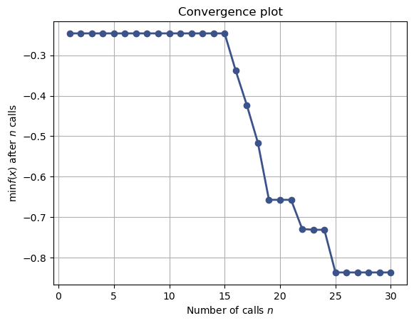
from skopt.plots import plot_convergence
plot_convergence(res);
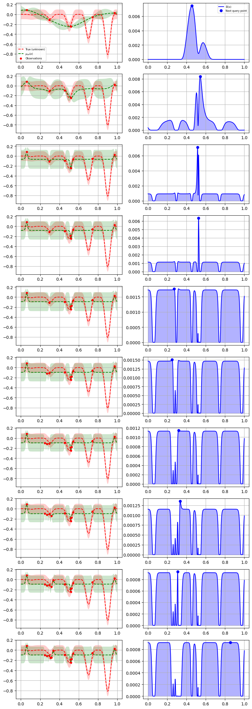
from skopt.plots import plot_gaussian_process
for n_iter in range(10):
# Plot true function.
plt.subplot(10, 2, 2 * n_iter + 1)
if n_iter == 0:
show_legend = True
else:
show_legend = False
ax = plot_gaussian_process(
res,
n_calls=n_iter,
objective=lambda x: objective(x, 0),
noise_level=0.05,
show_legend=show_legend,
show_title=False,
show_next_point=False,
show_acq_func=False,
)
ax.set_ylabel("")
ax.set_xlabel("")
# Plot EI(x)
plt.subplot(10, 2, 2 * n_iter + 2)
ax = plot_gaussian_process(
res,
n_calls=n_iter,
show_legend=show_legend,
show_title=False,
show_mu=False,
show_acq_func=True,
show_observations=False,
show_next_point=True,
)
ax.set_ylabel("")
ax.set_xlabel("")
fig = plt.gcf()
fig.set_figheight(30)
fig.set_figwidth(10)
plt.show()
Let’s compare this to our much simpler sampling strategies!
fig = go.Figure()
fig.add_scatter(
x=df_random["num_samples"],
y=df_random["objective"],
# error_y={"array": df_random["stdev"]},
name="Random sampling",
)
fig.add_scatter(
x=df_latinhypercube["num_samples"],
y=df_latinhypercube["objective"],
# error_y={"array": df_latinhypercube["stdev"]},
name="Latin Hypercube Sampling",
)
fig.add_scatter(
x=df_sobol["num_samples"],
y=df_sobol["objective"],
# error_y={"array": df_sobol["stdev"]},
name="Sobol sampling",
)
fig.add_scatter(
x=list(range(len(res.func_vals))),
y=np.maximum.accumulate(-res.func_vals),
name="scikit-optimize",
)
In-class experiment: paper helicopters!#
We will demonstrate DoE starting from scratch for a physical system using an online service (SigOpt, now a subsidiary of Intel) to optimize a number of parameters for paper helicopter flight time! This demonstration will show:
how DoE can be used in real life
parameter constraints
uncertainty in experimental data
analysis and visualization of high dimension experiments
SigOpt takes care of many of the details of actually building a predictive model for your data. They make this process very straightforward. There are many open source alternatives that could also be used, but they take a bit more time to learn/use:
hyperopt
scikit-optimize
ax
gpyopt
wandb
…
Spreadsheet for the experiments for this class! (CMU access only, so use your CMU google account) https://docs.google.com/spreadsheets/d/1Is9t9-sknFipdiN5MvuOyMCScjjv2JXGu0Ou4Gzlh_g/edit#gid=0