\[\newcommand{\arr}[1]{\underline{\underline{#1}}}\]

\[\newcommand{\vec}[1]{\underline{#1}}\]

\[\require{mhchem}\]

Application of linear ODEs to ChE examples

Alternate Method (Last class continued)

Treat as Linear ODE

(181)\[\begin{align} \frac{dC}{dt} = \frac{F}{V}C_{in} - \frac{1}{V}(F+kV)C\\ \frac{dC}{dt} + \frac{1}{V} (F+kV)C = \frac{F}{V}C_{in} \end{align}\]

Take \(p(t) = \frac{1}{V}(F+kV)\) and \(r(t) = \frac{F}{V}C_{in}\). Then,

(182)\[\begin{align} h &= \int p(t)dt\\ &= \int \frac{1}{V}(F+kV)dt = \frac{F+kV}{V}t \end{align}\]

And

(183)\[\begin{align} C(t) &= e^{-h}\left[\int e^h r(t)dt + \alpha \right]\\ &= e^{-h}\left[\int e^h \frac{F}{V}C_{in}dt + \alpha \right]\\ &= e^{-h}\left[ \frac{F}{V}C_{in}\int \exp \left(\frac{F+kV}{V}t \right) dt + \alpha \right]\\ &= e^{-h}\left[ \frac{F}{V}C_{in} \cdot \frac{V}{(F+kV)} \exp \left(\frac{F+kV}{V}t \right) + \alpha \right]\\ C(t) &= \frac{F C_{in}}{F+kV} + \alpha \exp \left[\frac{-(F+kV)}{V}t \right] && \text{general solution} \end{align}\]

If \(C(t=0) = C_0\) then \(C_0 = \frac{FC_{in}}{F+kV} + \alpha \implies \alpha = C_0 - \frac{FC_{in}}{F+kV}\) and

(184)\[\begin{align} C(t) = \frac{FC_{in}}{F+kV} \left(1 - \exp \left[\frac{-(F+kV)}{V}t \right] \right) + C_0 \exp \left[\frac{-(F+kV)}{V}t \right] && \text{specific solution} \end{align}\]

• Since we were able to solve both as separable and linear, why would we deal with linear?

Solutions with time varying (but known) feed concentrations)

• There will be some cases where we must:
  \(\implies\) What if the feed concentration varies with time for the same example?

(185)\[\begin{align} \text{Accum = In - Out + Gen - Consumption}\\ \frac{dM}{dt} = V\frac{dC}{dt} = FC_f(t) - FC(t) - kVC(t)\\ \frac{dC}{dt} + \left(\frac{F+kV}{V} \right)C = \frac{F}{V}C_F(t) && \text{(not separable)} \end{align}\]

Take \(p(t) = \left(\frac{F+kV}{V} \right)\) and \(r(t) = \frac{F}{V}C_F(t)\)
\(\rightarrow\) Solve as a linear \(1^\circ\) ODE:

(186)\[\begin{align} h \equiv \int p(t)dt = \int \frac{F+kV}{V}dt = \left( \frac{F+kV}{V}\right)t = \alpha t \end{align}\]

then,

(187)\[\begin{align} C(t) &= e^{-h} \left(\int e^h \cdot r(t)dt + N \right)\\ C(t) &= e^{-\alpha t}\left( \frac{F}{V}\int e^{\alpha t} \cdot C_F(t) dt + N\right) \end{align}\]

\(\rightarrow\) need to know \(C_F(t)\) to solve. Let’s consider several cases:

No feed (\(C_F(t) = 0\))

\(\underline{\text{Case 1:}}\) \(C_F(t) = 0 \rightarrow\) no feed

• Think first: tank is filled with initial reactant at \(C_0\) and that’s all there will be. Solution for \(C(t)\) should decay from \(C_0\) to 0.

(188)\[\begin{align} C(t) &= e^{-\alpha t} \left(\frac{F}{V}\int e^{\alpha t} \cdot 0 \cdot dt + N \right) \\ &= Ne^{-\alpha t} \end{align}\]

then, \(C(t=0)=C_0=Ne^{-\alpha 0} \implies N=C_0\) and

(189)\[\begin{align} C(t) = C_0 e^{-\alpha t} \end{align}\]

Constant feed (\(C_F(t) = C_F\))

\(\underline{\text{Case 2:}}\) \(C_F(t) = C_F \rightarrow\) constant feed

• Think first: initial conc. in tank is \(C_0\) and will assyptotically approach a lower or highr value depending on if \(C_F<C_0\) or \(C_F>C_0\)

(190)\[\begin{align} C(t) &= e^{-\alpha t}\left(\frac{F}{V} \int e^{\alpha t} \cdot C_F dt + N \right)\\ &= e^{-\alpha t} \left(\frac{FC_F}{V\alpha}e^{\alpha t} + N \right)\\ C(t) &= \frac{FC_F}{V\alpha} + N e^{-\alpha t} \end{align}\]

then, \(C(t=0) = C_0 = \frac{FC_F}{V\alpha} + N e^{-\alpha 0} \implies N = C_0 - \frac{FC_F}{V\alpha}\) and

(191)\[\begin{align} C(t) &= \frac{FC_F}{V\alpha} + \left(C_0 - \frac{FC_F}{V\alpha} \right) e^{-\alpha t}\\ C(t) &= \frac{FC_F}{V\alpha} (1 - e^{-\alpha t}) + C_0 e^{-\alpha t} \end{align}\]

At steady state:

(192)\[\begin{align} C(t) \lim_{t \rightarrow \infty} = \frac{FC_F}{V \alpha} = \frac{FC_F}{F+kV} \end{align}\]

Exponentially decaying feed (\(C_F(t) = C_F \exp(-\beta t)\))

\(\underline{\text{Case 3}}\) : \(C_F(t) = C_F \exp(-\beta t)\) (decaying function)

\(\beta\) controls the speed of the approach to steady state

(193)\[\begin{align} C(t) &= e^{-\alpha t}\left(\frac{F}{V} \int e^{\alpha t} \cdot C_F \cdot e^{-\beta t}dt + N \right)\\ &= e^{-\alpha t}\left(\frac{FC_F}{V} \int e^{(\alpha - \beta) t} dt + N \right)\\ &= e^{-\alpha t}\left(\frac{FC_F}{V(\alpha - \beta)} e^{(\alpha - \beta) t} + N \right)\\ &= \frac{FC_F}{V(\alpha - \beta)}e^{-\beta t} + N e^{-\alpha t} \end{align}\]

then \(C(t=0) = C_0 = \frac{FC_F}{V(\alpha - \beta)}e^0 + Ne^0 \implies N = C_0 - \frac{FC_F}{V(\alpha - \beta)}\) and

(194)\[\begin{align} C(t) = \frac{FC_F}{V(\alpha - \beta)} e^{-\beta t} + \left(C_0 - \frac{FC_F}{V(\alpha - \beta)} \right) e^{-\alpha t} \end{align}\]

At steady state,

(195)\[\begin{align} C(t) \lim_{t \rightarrow \infty} = 0 \end{align}\]

Makes sense, right? No new reactant entering the reactor at steady state Rate of decay depends on parameters \(\alpha, \beta, V, C_f\) and \(F\)

Oscillating Feed (\(C_F(t) = C_f[1+\sin(\omega t)]\)(

\(\underline{\text{Case 4}}\): \(C_F(t) = C_f[1+\sin(\omega t)]\) (oscillating feed)

(196)\[\begin{align} C(t) &= e^{-\alpha t} \left[\frac{F}{V}\int e^{\alpha t} \cdot C_F [1+\sin(\omega t)] dt + N \right]\\ &= e^{-\alpha t} \left[\frac{FC_F}{V}\int (e^{\alpha t} + e^{\alpha t} \sin(\omega t)) dt + N \right]\\ &= e^{-\alpha t}\left[\frac{FC_F}{\alpha V} e^{\alpha t} + \frac{FC_F}{V(\alpha^2 + \omega^2)} e^{\alpha t} (\alpha \sin \omega t - \omega \cos \omega t) \right]\\ &= \frac{FC_F}{\alpha V} + \frac{FC_F}{V(\alpha^2 + \omega^2)}[\alpha \sin(\omega t)-\omega \cos(\omega t)] + Ne^{-\alpha t} \end{align}\]

then

(197)\[\begin{align} C(t=0) = C_0 &= \frac{FC_F}{\alpha V} + \frac{FC_F}{V(\alpha^2 + \omega^2)} \cdot (-\omega) + Ne^0\\ N &= C_0 - \frac{FC_F}{V} \left(\frac{1}{\alpha} - \frac{\omega}{\alpha^2 + \omega^2} \right) \end{align}\]

and:

(198)\[\begin{align} C(t) = \frac{F}{V}C_F \left[\frac{1}{\alpha} + \frac{\alpha \sin \omega t - \omega \cos \omega t}{\alpha^2 + \omega ^2} \right] + \left[C_0 - \frac{F}{V}C_F \left(\frac{1}{\alpha} - \frac{\omega}{\alpha^2 + \omega^2} \right) \right]e^{-\alpha t} \end{align}\]

At steady state right side term drops out; we’r still oscillating at steady state.

Numerical evaluation of the solutions to an oscillatory CSTR feed

Simplest way using constants for the parameters

import numpy as np
import matplotlib.pyplot as plt

F = 1
V = 1
k = 1
omega = 1
Cf = 2
C0 = 4

alpha = (F+k*V)/V

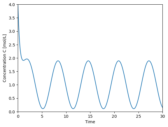
t = np.linspace(0,30,500)

C = F/V*Cf*(1/alpha + \
            (alpha*np.sin(omega*t)-omega*np.cos(omega*t))/(alpha**2+omega**2)) + \
            (C0-F/V*Cf*(1/alpha-omega/(alpha**2+omega**2)))*np.exp(-alpha*t)

plt.plot(t,C)
plt.xlabel('Time')
plt.ylabel('Concentration C [mol/L]')
plt.xlim([0,30])
plt.ylim([0,4])

(0.0, 4.0)

alpha

2.0

omega

1

More readable/helpful way using a function to do the solution; this way we know exactly what the parameters are that can be varied, and we can set defaults for parameters. This makes plotting for different parameters really clean!

import numpy as np
import matplotlib.pyplot as plt

def solve_C(t, 
            V = 1, 
            F = 1, 
            k = 1, 
            omega = 1, 
            Cf = 2, 
            C0 = 4):
  
  # This function evaluates the solution for a CSTR with a time-varying 
  # sinusoidal feed concentration
  
  alpha = (F+k*V)/V

  C = F/V*Cf*(1/alpha + \
            (alpha*np.sin(omega*t)-omega*np.cos(omega*t))/(alpha**2+omega**2)) + \
            (C0-F/V*Cf*(1/alpha-omega/(alpha**2+omega**2)))*np.exp(-alpha*t)
  return C


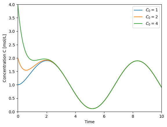
t = np.linspace(0,10,500)

plt.plot(t,solve_C(t=t, C0=1), label='$C_0=1$') 
plt.plot(t,solve_C(t=t, C0=2), label='$C_0=2$') 
plt.plot(t,solve_C(t=t, C0=4), label='$C_0=4$') 

plt.xlabel('Time')
plt.ylabel('Concentration C [mol/L]')
plt.xlim([0,10])
plt.ylim([0,4])
plt.legend()

<matplotlib.legend.Legend at 0x7f5f18432770>

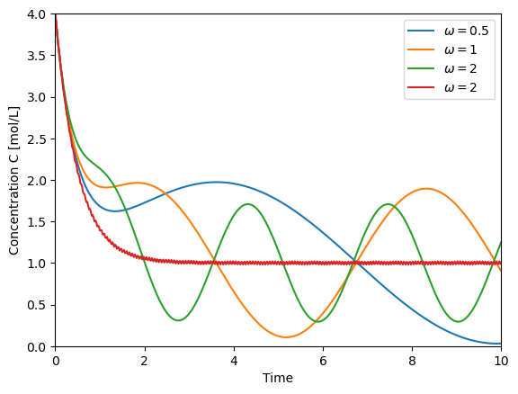
t = np.linspace(0,10,500)

plt.plot(t,solve_C(t=t, omega=0.5), label='$\omega=0.5$') 
plt.plot(t,solve_C(t=t, omega=1), label='$\omega=1$') 
plt.plot(t,solve_C(t=t, omega=2), label='$\omega=2$') 
plt.plot(t,solve_C(t=t, omega=100), label='$\omega=2$') 

plt.xlabel('Time')
plt.ylabel('Concentration C [mol/L]')
plt.xlim([0,10])
plt.ylim([0,4])
plt.legend()

<matplotlib.legend.Legend at 0x7f5f3b5f3580>

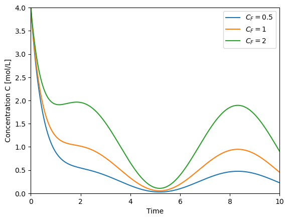
t = np.linspace(0,10,500)

plt.plot(t,solve_C(t=t, Cf=0.5), label='$C_F=0.5$') 
plt.plot(t,solve_C(t=t, Cf=1), label='$C_F=1$') 
plt.plot(t,solve_C(t=t, Cf=2), label='$C_F=2$') 

plt.xlabel('Time')
plt.ylabel('Concentration C [mol/L]')
plt.xlim([0,10])
plt.ylim([0,4])
plt.legend()

<matplotlib.legend.Legend at 0x7f5f1826d1b0>