\[\newcommand{\arr}[1]{\underline{\underline{#1}}}\]

\[\newcommand{\vec}[1]{\underline{#1}}\]

\[\require{mhchem}\]

Boundary value problems

Everything so far: Initial value problems

• Initial conditions specify state at a single value of the independent variable

(473)\[\begin{align} t = 0 \rightarrow y(t&=0) = y_0\\ y'(t&=0) = y_0' \end{align}\]

These IVP will have one unique solution. Implicitly, we have assumed that y and y’ are both defined at the initial condition, and that the system of differential equations is continuous over the solution interval.

\(\underline{\text{Ex}}\): \(y'' = 0 \hspace{2cm} y(0) = 2, \ y'(0) = 1\)

(474)\[\begin{align} y(t) = ct + d\\ y(0) = 2 = d && \rightarrow \text{IC#1 gives intercept}\\ y'(0) = 1 = c && \text{IC#2 gives slope} \end{align}\]

If we know information at two different points in the independent variable, we have a boundary value problem.

Example: pirate defense

1. Analytical solution \(\rightarrow\) apply all of our boundary conditions

(475)\[\begin{align} \frac{d}{dt}\begin{bmatrix}x\\z\\v_x\\v_z \end{bmatrix} = \begin{bmatrix} v_x\\v_z\\-rv_x\\-rv_z-g\end{bmatrix} \rightarrow \text{physics with air friction} \end{align}\]

(476)\[\begin{align} x(t=0) = 0\\ z(t=0) = H\\ z(x=L) = 0 \end{align}\]

That third condition is very strange!

The conditions that we would use if we were treating this as an initial value problem are:

(477)\[\begin{align} x(t=0) = 0\\ z(t=0) = H\\ v_x(t=0) = ?\\ v_z(t=0) = ? \end{align}\]

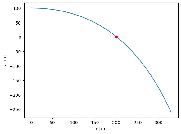
Say we are firing from a 100m embankment and the pirate ship is 200m away. We want to find initial conditions for \(v_x\) and \(v_z\) such that we hit the pirate ship. Code this up and let’s discuss. g = 9.8 [m/s^2] and r=0.1 [1/s]. Go ahead and try to solve this, starting from t=0 and integrating for 10 seconds.

import numpy as np
import matplotlib.pyplot as plt
from scipy.integrate import solve_ivp

r = 0.1 #1/s
g = 9.8 #m/s^2
H = 100 # m
L = 200 # m

def diff_eq(t, y):
  x, z, vx, vz = y
  return [vx,
          vz,
          -r*vx,
          -r*vz-g]

y0 = [0,
      H,
      52, #m/s
      0] #m/s

t_span = [0,10]
t_eval = np.linspace(0,10,100)

sol = solve_ivp(diff_eq,
                t_span=t_span,
                y0=y0,
                t_eval=t_eval)

plt.plot(sol.y[0,:],
         sol.y[1,:])
plt.plot(200,0,'or')
plt.xlabel('x [m]')
plt.ylabel('z [m]')

Text(0, 0.5, 'z [m]')

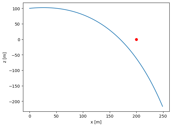
Say that we know that the cannonballs were fired at a speed of 40 m/s, but the angle of firing could be adjusted (e.g. \(v_x=v\cos \theta, v_z=v\sin\theta\)). Is it possible to hit the pirate ship?

import numpy as np
import matplotlib.pyplot as plt
from scipy.integrate import solve_ivp

r = 0.1 #1/s
g = 9.8 #m/s^2
H = 100 # m
L = 200 # m

def diff_eq(t, y):
  x, z, vx, vz = y
  return [vx,
          vz,
          -r*vx,
          -r*vz-g]

v0 = 40 # m/s
theta = 10 # degree
y0 = [0,
      H,
      v0*np.cos(theta/360*2*np.pi), #m/s
      v0*np.sin(theta/360*2*np.pi)] #m/s

t_span = [0,10]
t_eval = np.linspace(0,10,100)

sol = solve_ivp(diff_eq,
                t_span=t_span,
                y0=y0,
                t_eval=t_eval)

plt.plot(sol.y[0,:],
         sol.y[1,:])
plt.plot(200,0,'or')
plt.xlabel('x [m]')
plt.ylabel('z [m]')

Text(0, 0.5, 'z [m]')

So, what did we learn?

• Sometimes there is a solution for BVPs

• Sometimes there are multiple solutions

• Sometimes there are no solutions

• There could even be infinite solutions

Analytical solutions to BVPs

Analytical solutions to BVPs are usually not a problem to solve, just new boundary conditions.

\(\underline{\text{Ex}}\): \(2^{nd}\) order ODE would be specified by

(478)\[\begin{align} y(x=x_1) = y_1\\ y(x=x_2) = y_2 \end{align}\]

Can have

• no solutions

• one solution

• infinite solutions

\(\underline{\text{Ex}}\):

(479)\[\begin{align} y'' + \lambda y = 0 && \rightarrow \text{rod of length $L$}\\ y(0) = 0\\ y(L) = 0 \end{align}\]

\begin{equation} y(x)=\begin{cases} A\cos\sqrt{\lambda}x + B \sin\sqrt{\lambda}x & \lambda \neq 0\\ cx + d & \lambda = 0 \end{cases} \end{equation} * If $\lambda = 0$, only $c,d$ allowed with boundary conditions is trivial solution * If $\lambda \neq 0$ and $A$ or $B$ not 0, $y(x) = B\sin\sqrt{\lambda}x$ is a solution only if $\lambda = \left(\frac{n\pi}{L}\right)^2\rightarrow$ infinite number of solutions

Example BVP:

If we apply axial load or pressure, we will eventually have a buckle

As engineers, we care about shape

• Also care about critical \(P\)

(480)\[\begin{align} EIy'''' + Py'' = 0 \end{align}\]

BC:

(481)\[\begin{align} y(x=0) = 0 && y'(x=L) = 0\\ y(x=L) = 0 && y''(x=0) = 0 \end{align}\]

(482)\[\begin{align} y'''' + \lambda y'' = 0 && \lambda \equiv \frac{P}{EI}\\ F \equiv y'' \rightarrow && F'' + \lambda F = 0 \end{align}\]

Two cases!

1. \(\lambda = 0\)

\[\begin{align*} \int y'''' &= \int 0 \\ \int y''' &= \int a \\ y'' &= ax + b\\ y &= c_1x^3 + c_2x^2 + c_3x + c_4 \end{align*}\]

apply BC:

(483)\[\begin{align} y(c&=0) = 0 = c_4\\ y''(x&=0) = 0 = 2c_2\\ y(x&=L) = 0 = c_1L^3 + c_3L \rightarrow c_3 = -c_1L^2\\ y'(x&=L) = 0 = 3c_1L^2 + c_3 \rightarrow c_1 = 0 = c_3 \end{align}\]

For \(\lambda = 0, \ y(x) = 0 \rightarrow\) trivial / no solution
This is the solution if \(P=0\) 2. \(\lambda \neq 0 \rightarrow y'''' + \lambda y'' = 0\)
guess \(y(x) = e^{rx}\)
plug in:

(484)\[\begin{align} r^4e^{rx} + \lambda r^2e^{rx} = 0\\ r^4 + \lambda r^2 = 0\\ r^2(r^2 + \lambda) = 0\\ r = 0,\ 0,\ \pm i\sqrt{\lambda} \\ \end{align}\]

(485)\[\begin{align} y_1 &= e^{0x}\\ y_2 &= xe^{0x}\\ y_3 &= \sin\sqrt{\lambda}x\\ y_4 &= \cos\sqrt{\lambda}x \end{align}\]

(486)\[\begin{align} y(x) &= c_1 + c_2x + c_3\sin\sqrt{\lambda}x + c_4\cos\sqrt{\lambda}x\\ y'(x) &= c_2 + c_3\sqrt{\lambda}\cos\sqrt{\lambda}x - c_4\sqrt{\lambda}\sin\sqrt{\lambda}x\\ y''(x) &= -c_3\lambda\sin\sqrt{\lambda}x - c_4\lambda\cos\sqrt{\lambda}x \end{align}\]

BC:

1.\begin{align} y(x=0) = 0 = c_1 + c_4 \end{align} 2.\begin{align} y’’(x=0) = 0 = -c_4 \lambda \rightarrow c_4 = 0, \ c_1 = 0 \end{align} 3.\begin{align} y(x=L) = 0 &= c_2L + c_3\sin\sqrt{\lambda}L\ c_2 & = -\frac{1}{L}c_3\sin\sqrt{\lambda}L \end{align} 4.\begin{align} y’(x=L) = 0 &= c_2 + c_3\sqrt{\lambda}\cos\sqrt{\lambda}L\ 0 &= -\frac{1}{L}c_3\sin\sqrt{\lambda}L + c_3\sqrt{\lambda}\cos\sqrt{\lambda}L\ &= c_3(\sqrt{\lambda}L\cos\sqrt{\lambda}L - \sin\sqrt{\lambda}L) \end{align} Only situation without trivial solution is if

(487)\[\begin{align} \sqrt{\lambda}L\cos\sqrt{\lambda}L - \sin\sqrt{\lambda}L = 0\\ \rightarrow \tan\sqrt{\lambda}L = \sqrt{\lambda}L \rightarrow \tan x = x \end{align}\]

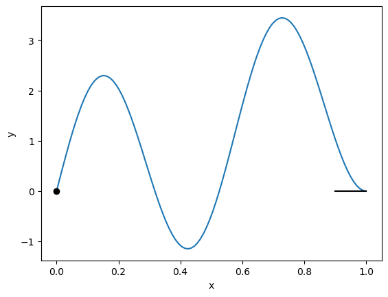
\(\rightarrow\) infinite number of solutions but only care about the first one (smallest \(P\))

(488)\[\begin{align} \sqrt{\lambda}L &= 4.4934...\\ \lambda_1 &= \frac{(4.493)^2}{L^2}\\ P &= \lambda EI \rightarrow P_{max} = \frac{(4.49)^2}{L^2}EI \approx \frac{20.2}{L^2}EI \end{align}\]

from scipy.optimize import root
import numpy as np
import matplotlib.pyplot as plt

L = 1
sol = root(lambda x: np.tan(x)-x, 4+np.pi*4)

rootLambdaL = sol.x
lambdaSol = (rootLambdaL/L)**2

c3 = 2
c2 = -c3*np.sin(np.sqrt(lambdaSol)*L)/L

xrange = np.linspace(0,L,100)
plt.plot(xrange,
         c2*xrange+c3*np.sin(np.sqrt(lambdaSol)*xrange))

plt.plot(0,0,'ok')
plt.plot([0.9,1],[0,0],'-k')
plt.xlabel('x')
plt.ylabel('y')

Text(0, 0.5, 'y')

plt.xlabel('x')

Text(0.5, 0, 'x')