\[\newcommand{\arr}[1]{\underline{\underline{#1}}}\]

\[\newcommand{\vec}[1]{\underline{#1}}\]

\[\require{mhchem}\]

Coupled Differential Equations

• Everything we’ve done so far has involved functions that depend only on independent variables:
  e.g.,

(371)\[\begin{align} y(x) && or && y(x,t)\\ \frac{dy}{dx} \text{ for ODEs } && && \frac{\partial y}{\partial x} \& \frac{\partial y}{\partial t} \text{ for PDEs} \end{align}\]

• Sometimes, functions can depend on other functions. e.g. given \(y_1(x)\) & \(y_2(x)\)

(372)\[\begin{align} \frac{dy_1}{dx} = y_2\\ \frac{dy_2}{dx} = y_1 + \sin x \end{align}\]

are coupled ODEs. Sometimes, we can solve by substitution (e.g. take derivative of equation 1 above and substitute into equation 2) but often will want/need to solve simultaneously.

Chemical Engineering Example

Tanks in series example

(373)\[\begin{align} F_1 &= \frac{h_1 - h_2}{R_1}\\ F_{out} &= \frac{h_2}{R_2} \end{align}\]

• No feed to first tank; \(F_1\) and \(F_{out}\) are volumetric flow rates controlled by resistance valves and are proportional to water height in each tank ( which is a function of time)

• System is coupled because \(F_1\) depends on both \(h_1(t)\) and \(h_2(t)\).
  Tank 1 MB:

(374)\[\begin{align} \frac{dM}{dt} &= -\rho \cdot F_1 && \left[ \frac{kg}{s} \right] = \left[\frac{kg}{m^3} \right] \cdot \left[\frac{m^3}{s} \right]\\ \rho A_1 \frac{dh_1}{dt} &= -\rho \left(\frac{h_1 - h_2}{R_1} \right) && \left[\frac{kg}{m^3} \right] \cdot [m^2] \cdot \left[\frac{m}{s} \right] = \left[\frac{kg}{s} \right]\\ \frac{dh_1}{dt} &= \frac{h_2}{\tau_1} - \frac{h_1}{\tau_1} \end{align}\]

where \(\tau \equiv A_iR_i \ [=] \ time\) is the “residence time”
Tank 2 MB:

(375)\[\begin{align} \rho A_2 \frac{dh_2}{dt} &= \rho(F_1 - F_{out})\\ \frac{dh_2}{dt} &= \frac{1}{A_2} \left( \frac{h_1 - h_2}{R_1} - \frac{h_2}{R_2}\right)\\ &= \frac{R_2}{\tau_2}\left( \frac{h_1 - h_2}{R_1} - \frac{h_2}{R_2}\right)\\ &= \frac{R_2h_1}{R_1\tau_2} - \frac{R_2h_2}{R_1\tau_2} - \frac{h_2}{\tau_2}\\ \frac{dh_2}{dt} &= \frac{R_2}{R_1\tau_2}h_1 - \frac{1}{\tau_2}\left(1 + \frac{R_2}{R_1} \right)h_2 \end{align}\]

Convert two first-order diff eq to a second order diff eq

One approach you can take is to calculate the derivative of the \(1^{st}\) MB and using it to eliminate \(h_2(t)\)

(376)\[\begin{align} \frac{d^2h_1}{dt^2} &= \frac{1}{\tau_1}\frac{dh_2}{dt} - \frac{1}{\tau_1}\frac{dh_1}{dt}\\ \frac{dh_2}{dt} &= \tau_1 \frac{d^2h_1}{dt^2} + \frac{dh_1}{dt} \end{align}\]

And (from the \(1^{st}\) MB):

(377)\[\begin{align} h_2 = \tau_1 \frac{dh_1}{dt} + h_1 \end{align}\]

• Plug those into MB #2

(378)\[\begin{align} \tau_1 \frac{d^2h_1}{dt^2} + \frac{dh_1}{dt} = \frac{R_2}{R_1\tau_2}h_1 - \frac{1}{\tau_2}\left(1 + \frac{R_2}{R_2} \right)\left(\tau_1 \frac{dh_1}{dt} + h_1 \right) \end{align}\]

simplify:

(379)\[\begin{align} h_1'' + \left(\frac{\tau_2 + \tau_1 + \frac{R_2}{R_1}\tau_1}{\tau_1\tau_2} \right) h_1' + \frac{1}{\tau_1\tau_2}h_1 = 0 \end{align}\]

• whew! Now we need to solve for \(h_1(t)\) and then plug back in to find \(h_2(t)\)

• Too much work! Can we solve for \(h_1(t)\) and \(h_2(t)\) simultanously?

Solving as coupled differential equations

(380)\[\begin{align} h_1' &= -\frac{1}{\tau_1}h_1 + \frac{1}{\tau_1}h_2\\ h_2' &= \frac{R_2}{R_1\tau_2}h_1 - \left(1 + \frac{R_2}{R_1} \right)\frac{1}{\tau_2}h_2 \end{align}\]

• Now let’s set

(381)\[\begin{align} a_{11} = -\frac{1}{\tau_1} && a_{12} = \frac{1}{\tau_1}\\ a_{21} = \frac{R_2}{R_1\tau_2} && a_{22} = -\frac{1}{\tau_2}\left(1 + \frac{R_2}{R_1}\right) \end{align}\]

• Then we have:

(382)\[\begin{align} h_1' = a_{11}h_1 + a_{12}h_2\\ h_2' = a_{21}h_1 + a_{22}h_2 \end{align}\]

• Look familiar?

(383)\[\begin{align} \begin{bmatrix}h_1' \\ h_2' \end{bmatrix} &= \begin{bmatrix} a_{11} & a_{12} \\ a_{21} & a_{22}\end{bmatrix} \begin{bmatrix} h_1 \\ h_2 \end{bmatrix}\\ \vec{h'} = \arr{A} \vec{h} \end{align}\]

• Let’s foray into derivative matrices before returning to our tank problem
  Property:

(384)\[\begin{align} \begin{bmatrix}\frac{dy_1}{dt} \\ \frac{dy_2}{dt} \end{bmatrix} = \begin{bmatrix} y_1' \\ y_2' \end{bmatrix} = \frac{d}{dt}\begin{bmatrix}y_1 \\ y_2 \end{bmatrix} \rightarrow \text{take derivative of each element} \end{align}\]

Vector derivative example

\(\underline{\text{Ex}}\): If \(\vec{y}(x) = \begin{bmatrix}4t & 3t^2 \\ 2t^3 & t \end{bmatrix}\)

\(\vec{y'}(x) = \begin{bmatrix}4 & 6t \\ 6t^2 & 1 \end{bmatrix}\)

Continuing!

• Goal is to solve \(\vec{y'} = \frac{d}{dt} \vec{y} = \arr{A}\vec{y}\) for \(\vec{y}(t)\)

(385)\[\begin{align} \begin{bmatrix}y_1' \\ y_2' \end{bmatrix} = \begin{bmatrix} a_{11} & a_{12} \\ a_{21} & a_{22} \end{bmatrix} \begin{bmatrix} y_1 \\ y_2\end{bmatrix} \end{align}\]

\(y_1(t)\) and \(y_2(t)\) are coupled functions, not basis functions.

• Let’s assume \(\vec{y}\) takes the form \(\vec{y} = \vec{x}e^{\lambda t}\) wher \(\vec{x}\) is a vector of constants

(386)\[\begin{align} \therefore \vec{y'} = \lambda \vec{x}e^{\lambda t} \end{align}\]

• Plugging back into \(\vec{y'} = \arr{A}\vec{y}\) gives

(387)\[\begin{align} \lambda \vec{x} e^{\lambda t} &= \arr{A}\vec{x}e^{\lambda t}\\ \lambda \vec{x} &= \arr{A}\vec{x} \end{align}\]

\(\therefore\)Any set of \(y_1(t) = x_1e^{\lambda t}\) and \(y_2(t) = x_2e^{\lambda t}\) that fits \(\lambda\vec{x} = \arr{A} \vec{x}\) are solutions. Therefore, finding the eigenvalues and eigenvectors of \(\arr{A}\) will yield solution.

Example

(388)\[\begin{align} y_1' &= -4y_1 - 6y_2\\ y_2' &= y_1 + y_2 \end{align}\]

• By assuming that \(\vec{y} = \vec{x}e^{\lambda t}\), we can find the eigenvalues and vectors of \(\arr{A}\) to identify \(\vec{x}\) and \(\lambda\) to solve system.

• Find \(\lambda\) and \(\vec{x}\) by solving

(389)\[\begin{align} \det(\arr{A} - \lambda \arr{I}) = 0\\ \left|\begin{array}{} -4-\lambda & -6 \\ 1 & 1-\lambda \end{array}\right| = 0\\ (-4-\lambda)(1-\lambda) - (-6)(1) = 0\\ -4 + 3\lambda + \lambda^2 + 6 = 0 \\ \lambda^2 + 3\lambda + 2 = 0&& \leftarrow \text{char. eqn. of $\arr{A}$}\\ (\lambda + 2)(\lambda + 1) = 0\\ \lambda_1 = -2; \hspace{0.5cm} \lambda_2 = -1 && \leftarrow \text{eigenvalues} \end{align}\]

• Find eigenvector \(\vec{x}^{(1)}\) associated with \(\lambda_1 = -2\).
  solve

(390)\[\begin{align} \arr{A}\vec{x}^{(1)} = \lambda_1 \vec{x}^{(1)}\\ (\arr{A} - \lambda_1\arr{I}) \vec{x}^{(1)} = \vec{0}\\ \begin{bmatrix}-2 & -6 \\ 1 & 3 \end{bmatrix} \begin{bmatrix}x_1 \\ x_2 \end{bmatrix} = \begin{bmatrix} 0 \\ 0 \end{bmatrix} \implies x_1 + 3x_2 = 0 \end{align}\]

Set \(x_1 = 1\) (arbitrary) then \(x_2 = -\frac{1}{3}\)
\(\therefore \vec{x}^{(1)} = \begin{bmatrix} 1 \\ -\frac{1}{3} \end{bmatrix}\) and \(\vec{y} = \begin{bmatrix} 1 \\ -\frac{1}{3}\end{bmatrix} e^{-2t}\) is a solution.
Enough?
No. Two coupled \(1^\circ\) ODEs will yield two solutions with two arbitrary constants.The rest of the solution comes from \(2^{nd}\) eigenvalue and eigenvector

• Find eigenvector \(\vec{x}^{(2)}\) associated with \(\lambda_2 = -1\)

(391)\[\begin{align} (\arr{A} - \lambda_2 \arr{I}) = \vec{0}\\ \begin{bmatrix}-3 & -6 \\ 1 & 2 \end{bmatrix} \begin{bmatrix} x_1 \\ x_2 \end{bmatrix} = \begin{bmatrix} 0 \\ 0 \end{bmatrix}\\ x_1 + 2x_2 = 0\\ \text{set } x_1 = 1\\ \therefore x_2 = -\frac{1}{2} \end{align}\]

\(\therefore x^{(2)} = \begin{bmatrix} 1 \\ -\frac{1}{2} \end{bmatrix} \) and \(\vec{y} = \begin{bmatrix} 1 \\ -\frac{1}{2} \end{bmatrix} e^{-t}\) is a solution

• The general solution to \(\vec{y}' = \arr{A}\vec{y}\) is

(392)\[\begin{align} \vec{y} &= c_1\vec{x}^{(1)} e^{\lambda_1t} + c_2\vec{x}^{(2)}e^{\lambda_2t}\\ \implies y_1 &= c_1e^{-2t} + c_2e^{-t}\\ y_2 &= -\frac{1}{3}c_1e^{-2t} - \frac{1}{2}c_2e^{-t} \end{align}\]

We have two constants in total from two integrations. We began with two \(1^\circ\) ODEs

• Let’s check our answer:

(393)\[\begin{align} y_1' &= -2c_1e^{-2t} - c_2e^{-t}\\ y_2' &= \frac{2}{3}c_1e^{-2t} + \frac{1}{2}c_2e^{-t} \end{align}\]

Plug into one original equation:

(394)\[\begin{align} y_1' &= -4y_1 - 6y_2\\ -2c_1e^{-2t} - c_2e^{-t} &= -4[c_1e^{-2t} + c_2e^{-t}] -6[-\frac{1}{3}c_1e^{-2t} - \frac{1}{2}c_2e^{-t}]\\ &= (-4+2)c_1e^{-2t} + (-4+3)c_2e^{-t}\\ &= -2c_1e^{-2t} - c_2e^{-t} \end{align}\]

And the other:

(395)\[\begin{align} y_2' &= y_1 + y_2\\ \frac{2}{3}c_1e^{-2t} + \frac{1}{2}c_2e^{-t} &= c_1e^{-2t} + c_2e^{-t} - \frac{1}{3}c_1e^{-2t}-\frac{1}{2}c_2e^{-t}\\ &= \frac{2}{3}c_1e^{-2t} + \frac{1}{2}c_2e^{-t} \end{align}\]

Now, let’s return to our tanks:
\(\vec{h}' = \arr{A}\vec{h}\) where

(396)\[\begin{align} \arr{A} = \begin{bmatrix} -\frac{1}{\tau_1} & \frac{1}{\tau_1} \\ \frac{R_2}{R_1\tau_2} & -\left(\frac{R_1 + R_2}{R_1\tau_2}\right) \end{bmatrix} \end{align}\]

• Assume solution of form \(\vec{h}= \vec{x}e^{\lambda t}\)

• Solve by inserting values for \(R_2,R_2,\tau_1\) and \(\tau_2 \rightarrow\) then find eigenvalues (\(\lambda_1\) and \(\lambda_2\)) and eigenvectors (\(\vec{x}^{(1)}\) and \(\vec{x}^{(2)}\)) of \(\arr{A}\)

• General solution will be

(397)\[\begin{align} \vec{h} &= c_1\vec{x}^{(1)}e^{\lambda_1t} + c_2\vec{x}^{(2)}e^{\lambda_2t}\\ \implies h_1(t) &= c_1x_1^{(1)}e^{\lambda_1t} + c_1x_1^{(2)}e^{\lambda_2t}\\ h_2(t) &= c_1x_2^{(1)}e^{\lambda_1t} + c_2x_2^{(2)}e^{\lambda_2t} \end{align}\]

For example, given:

(398)\[\begin{align} A_1 = 5\ m^2, R_1 = 2 \ hr/m^2 \rightarrow \tau_1 = 10\ hr\\ A_2 = 5 \ m^2, R_2 = 1 \ hr/m^2 \rightarrow \tau_2 = 5\ hr\\ \therefore \arr{A} = \begin{bmatrix} -0.1 & 0.1 \\ 0.1 & -0.3 \end{bmatrix} [=] \frac{1}{hr} \end{align}\]

• Find eigenvalues

(399)\[\begin{align} |\arr{A} - \lambda\arr{I}| = 0\\ \left|\begin{array}{} -0.1-\lambda & 0.1 \\ 0.1 & -0.3-\lambda \end{array}\right| = 0\\ (-0.1-\lambda)(-0.3-\lambda)-0.01 = 0\\ \lambda^2 + 0.4 \lambda + 0.02 = 0\\ \implies \lambda_1 = -0.06 \frac{1}{hr}\\ \lambda_2 = -0.34 \frac{1}{hr} &&\rightarrow \text{same units as $\arr{A}\hspace{1cm}$ ($\arr{A}\vec{x} = \lambda \vec{x}$)} \end{align}\]

• Find \(\vec{x}^{(1)}\) associated with \(\lambda_1 = -0.06 \ hr^{-1}\)

(400)\[\begin{align} \begin{bmatrix} -0.04 & 0.1 \\ 0.1 & -0.24 \end{bmatrix} \begin{bmatrix} x_1 \\ x_2 \end{bmatrix} = \begin{bmatrix} 0 \\ 0 \end{bmatrix}\\ \implies -0.04 x_1 + 0.1 x_2 = 0\\ x_1 = \frac{0.1}{+0.04}x_2 \simeq 2.5x_2 \implies \vec{x}^{(1)} \simeq \begin{bmatrix} 2.5 \\ 1 \end{bmatrix} \end{align}\]

• Find \(\vec{x}^{(2)}\) associated with \(\lambda_2 = -0.34\ hr^{-1}\)

(401)\[\begin{align} \begin{bmatrix} 0.24 & 0.1 \\ 0.1 & 0.04 \end{bmatrix} \begin{bmatrix} x_1 \\ x_2 \end{bmatrix} = \begin{bmatrix} 0 \\ 0 \end{bmatrix}\\ \implies 0.24 x_1 + 0.1 x_2 = 0\\ x_1 = \frac{0.1}{-0.24}x_2 \simeq -0.42x_2 \implies \vec{x}^{(2)} \simeq \begin{bmatrix} -0.42 \\ 1 \end{bmatrix} \end{align}\]

• General solution is:

(402)\[\begin{align} \vec{h} = c_1\begin{bmatrix}2.5 \\ 1 \end{bmatrix}e^{-0.06\ hr^{-1}t} + c_2 \begin{bmatrix} -0.42 \\ 1 \end{bmatrix} e^{-0.34\ hr^{-1}t} \end{align}\]

Numerical calculation of eigenvalues/eigenvectors

Remember we can get the eigenvectors/eigenvalues from scipy.

import numpy as np

# get the eigenvalues/eigenvectors and print them

# hint np.linalg.eig

A = np.array([[-0.1, 0.1],
              [0.1,-0.3]])

eigval, eigvec = np.linalg.eig(A)

print(eigval)
print(eigvec)

print(eigvec[:,0]/eigvec[1,0])

[-0.05857864 -0.34142136]
[[ 0.92387953 -0.38268343]
 [ 0.38268343  0.92387953]]
[2.41421356 1.        ]

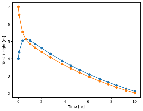
Numerical solutions to coupled differential equations

No real change from solve_ivp!

Try solving this with solve_ivp using the initial conditions \(h_1(t=0)=5\)m and \(h_2(t=0)=7\)m

from scipy.integrate import solve_ivp
import matplotlib.pyplot as plt
import numpy as np

A1 = 5 #m^2
R1 = 0.1 # hr/m^2
tau1 = A1*R1

A2 = 5 #m^2
R2 = 1 #hr/m^2
tau2 = A2*R2 

h0 = [4,7] #m

def hprime(t, h):
  A = np.array([[-1/tau1,1/tau1],
                [R2/R1/tau2,-1/tau2*(1+R2/R1)]])
  return A@h

sol = solve_ivp(hprime, [0,10], h0)

plt.plot(sol.t, sol.y.T,'o-')
plt.xlabel('Time [hr]')
plt.ylabel('Tank Height [m]')

Text(0, 0.5, 'Tank Height [m]')