\[\newcommand{\arr}[1]{\underline{\underline{#1}}}\]

\[\newcommand{\vec}[1]{\underline{#1}}\]

\[\require{mhchem}\]

Partial Differential Equations

• Function of interest depends on two or more independent variables \(\rightarrow\) typically time and one or more spatial variables.

• Only the simplest physical systems can be modeled by ODEs

• Most problems in science and engineering - including heat and mass transfer, fluid mechanics, quantum mechanics etc. lead to PDEs

Defining PDEs:

• Just like with ODEs, characterization of your PDE will indicate your solution method

• Order is defined by the order of the highest derivative

• A PDE is linear if it is of the first degree in the dependent variable and its partial derivatives.
  e.g.

(495)\[\begin{align} \frac{\partial^2u}{\partial x^2} &= \frac{\partial u}{\partial y} + u(x,y) && \text{linear}\\ \frac{\partial}{\partial x}\frac{\partial u}{\partial y} &= x^2 && \text{linear}\\ \frac{\partial u}{\partial x}\cdot \frac{\partial u}{\partial y} &= x^2 && \text{non-linear} \end{align}\]

• A linear PDE is homogeneous if every term contains the dependent variable or one of its derivatives
  Ex:

(496)\[\begin{align} \frac{\partial^2u}{\partial x^2} = \frac{\partial u}{\partial y} + x && \rightarrow \text{non-homogeneous} \end{align}\]

Notation

Often, \(u\) is the dependent variable; e.g. \(u=u(x,y,t)\)
\(\frac{\partial u}{\partial t}\) can be written as \(u_t\)
\(\frac{\partial^2u}{\partial x^2}\) can be written \(u_{xx}\)
\(\nabla u = \frac{\partial u}{\partial x} + \frac{\partial u}{\partial y} + \frac{\partial u}{\partial z}\)
\(\therefore\) if \(u_t = -c\nabla^2 u\)
\(\frac{\partial u}{\partial t} = -c \left[\frac{\partial^2u}{\partial x^2} + \frac{\partial^2u}{\partial y^2} + \frac{\partial^2u}{\partial z^2} \right]\)

Common PDE’s in Chemical Engineering

• There are many important linear PDEs of the second order in chemical engineering, particularly if you go to grad school. Some of the key equations are:

  1. Heat Transfer or diffusion
     A) \(u_t = c^2u_{xx} \rightarrow \) 1D \(\rightarrow u=u(t,x)\)
     B) \(u_t = c^2(u_{xx} + u_{yy})\rightarrow\) 2D; \(u = u(t,x,y)\)

  2. Wave equations

  • Arise in fields like accoustics, electromagnetics and fluid dynamics

  • Describe any kind of waves - mechanical (e.g. water, sound, seismic) or light waves
    A) \(u_{tt} = c^2u_{xx} \rightarrow\) 1D
    B) \(u_{tt} = c^2(u_{xx} + u_{yy}) \rightarrow\) 2D

  1. Laplace equation

  • Simplest example of an elliptic PDE (special type of linear second order PDE)

  • Solutions to these equations are the harmonic functions \(\rightarrow\) important in many fields of science - e.g. astronomy, electrostatics, fluid dynamics \(\rightarrow\) describe the behavior of fluid potentials ; also represents the steady state heat equation (no dependence on time)
    A) \(\nabla^2u = \Delta u = u_{xx} + u_{yy} = 0 \rightarrow\) 2D
    B) \(\nabla^2 u = \Delta u = u_{xx} + u_{yy} + u_{zz} = 0 \rightarrow\) 3D
    Here \(\Delta\) is the “Laplace operator”

Special Solutions to PDE’s

• There are often many possible general solutions to PDEs. For example, the 2D Laplace equation \(\nabla^2u = 0\) is satisfied by very unique functions:

(497)\[\begin{align} u(x,y) &= x^2 - y^2\\ u(x,y) &= e^x\cos y\\ \end{align}\]

In-class exercise

Is \(\ln(x^2+y^2)\) a solution to this differential equation?

Boundary/initial conditions in PDEs

• The particular solution for any problem is determined by boundary conditions and, if time is a variable, initial conditions.

  • Conditions must match up with the partial derivatives
    e.g. \(u_t = c^2u_{xx}\rightarrow\) requires 1 IC + 2 BC’s \(\rightarrow\) if you tried 2 IC’s and 1 BC, these would not be able to define the physical reality of the problem.

• Just as with ODEs, the superposition / linearity principle applies for linear PDE’s: if we have two linearly independent solutions of our PDE in some region \(R\), then the sum and linear combinations of those two solutions is also a solution \(\rightarrow\) if \(u_1\) and \(u_2\) are both solutions, then \(u_3 = c_1u_1 + c_2u_2\) is as well

Really simple linear PDEs:

\(\underline{\text{Ex}}\): \(u_{xx} - u = 0\)

• Since no derivatives w.r.t. \(y\) occur, we can solve like \(u'' - u = 0\), keeping in mind that our arbitrary constants will need to be functions of \(y\): \(\lambda^2 - 1 = 0\implies \lambda = \pm 1\)
  and \(u(x,y) = A(y)e^x + B(y) e^{-x}\)

\(\underline{\text{Ex}}\): \(u_{xy} = -u_x\)

• We can use reduction of order to simplify. Let \(p=u_x\). Then the PDE becomes

(498)\[\begin{align} \frac{\partial p}{\partial y} = -p \implies \frac{\partial p}{p} &= -dy\\ \ln p &= -y + \tilde{c}(x)\\ p(x,y) &= c(x)\exp(-y) \end{align}\]

And

(499)\[\begin{align} u_x=p\implies \frac{\partial u}{\partial x} &= c(x)\exp(-y)\\ u(x,y) &= e^{-y}\int c(x)dx + g(y) \rightarrow \text{arbitrary functions determined by two boundary conditions} \end{align}\]

Separation of Variables

• Method to solve some linear PDEs with linear boundary condtitions (heat equation, wave equation, laplace equation, Helmholtz equation, and others).

• Rests on the assumption that a multivariable function, like \(u(x,y,t)\) can be represented as a product of several single variable functions i.e. \(u(x,y,t) = X(x)Y(y)T(t)\)

• This will allow us to turn a PDE into two or more ODEs that we already know how to solve

• This does not always work, just like it didn’t always work for 1st order ODE’s

Worked Example: 1D Heat Transfer in a Bar

\(\underline{\text{Ex}}\): \(T_t(x) = \alpha T_{xx}\) (1D heat transfer)

Here \(\alpha\) is the thermal diffusivity with units of m\(^2\)/s. I’m solving this one in physical units, rather than the dimensionless forms above.

First, we assume \(T(x,t) = X(x) \cdot Y(t)\)

(500)\[\begin{align} \frac{\partial}{\partial t}(XY) &= \alpha \frac{\partial}{\partial x}\left( \frac{\partial(XY)}{\partial x}\right)\\ X\frac{dY}{dt} &= \alpha\frac{\partial}{\partial x}\left(Y\frac{dX}{dx} \right)\\ X\frac{dY}{dt} &= \alpha Y\frac{d^2X}{dx^2} && \text{now separate}\\ \frac{1}{Y}\frac{dY}{dt} &= \frac{\alpha}{X}\frac{d^2X}{dx^2} \end{align}\]

Call LHS = \(\frac{1}{Y}\frac{dY}{dt} = F(t)\) and RHS = \(\frac{\alpha}{X}\frac{d^2X}{dx^2} = G(x)\)
\(F(t)\) can equal \(G(x)\) only if both are equal to some constant, \(\mu\). One final note: \(\mu\) has units of 1/time as written.

Now, we can split our PDE into two ODEs

Solution for \(Y(t)\)

(501)\[\begin{align} \frac{1}{Y} \frac{dY}{dt} = \mu & \ \text{ separable $1^\circ$}\\ \int \frac{dY}{Y} = \int\mu dt\\ \ln Y = \mu t + c\\ Y(t) = c\exp(\mu t) \end{align}\]

At this point we haven’t know anything about \(\mu\). However, we can say that \(t\) should be

negative. If \(\mu\) was positive, we would have a temperature that explodes to \(\infty\), which is unphysical. To make things easier to see, I’m going replace \(\lambda=-\mu\). \(\lambda\) will be positive, but the exponential will tend to zero at long times.

\[\begin{align*} Y(t) = c\exp(\mu t) =c\exp(-\lambda t) \end{align*}\]

Solution for \(X(x)\)

(502)\[\begin{align} \frac{\alpha}{X}\frac{d^2X}{dx^2} = \mu=-\lambda \\ \frac{d^2X}{dx^2} + \frac{\lambda}{\alpha}X = 0 && \text{linear $2^\circ$ homogeneous constant coefficients} \end{align}\]

characteristic equation:

(503)\[\begin{align} r^2 + \frac{\lambda}{\alpha} = 0\\ r=\pm i\sqrt{\frac{\lambda}{\alpha}} \end{align}\]

Using Euler’s formula yields

(504)\[\begin{align} X = A\cos\sqrt{\frac{\lambda}{\alpha}}x + B\sin\sqrt{\frac{\lambda}{\alpha}}x \end{align}\]

1. Finally, the general solution is

(505)\[\begin{align} T(x,t) &= X(x)Y(t)\\ T(x,t) &= c\exp(-\lambda t)\left[A\cos\sqrt{\frac{\lambda}{\alpha}}x + B\sin\sqrt{\frac{\lambda}{\alpha}}x\right] \end{align}\]

Application of Boundary Conditions

A particular solution is identified by applying one IC and two BCs that represent the physical reality of the problem. Let’s assume the ends of the bar are held at a fixed reference temperature, which we will call 0 (this could be replaced by any constant \(T_{ref}\), since this is a linear equation).

(506)\[\begin{align} T(0,t) = 0 && T(L,t) = 0 && T(x,0)=f(x) \end{align}\]

We need three conditions because this is second order in \(x\) (need two conditions), and first order in \(t\) (need one initial condition). We’ll talk more about what this \(f(x)\) is.

1. BC #1: Apply \(T(0,t) = 0\)

\[\begin{align*} T(0,t) = 0 &= c \exp(-\lambda t)[A\cos(0) + B\sin(0)]=c \exp(-\lambda t)[A\cos(0)] \end{align*}\]

This whole thing has to be 0. \(c=0\) would only lead the trivial solution, so \(A\) has to be 0. 2. BC #2: \(T(L,t) = 0\)

\[\begin{align*} T(L,t) = 0 = ce^{-\lambda t} B\sin\left(\sqrt{\frac{\lambda}{\alpha}}L\right) \end{align*}\]

Again, we don’t want a trivial solution, so I want to pick \(\lambda\) such that the sin term is zero. This is only the case if

\[\begin{align*} \sqrt{\frac{\lambda}{\alpha}}L=n\pi \end{align*}\]

Solving for \(\lambda\):

\[\begin{align*} \lambda_n=\alpha\left(\frac{n\pi}{L}\right)^2 \end{align*}\]

This implies there’s actually a series of solutions The solution is then

\[\begin{align*} T(x,t)=c_ne^{-\lambda_n t} \sin\left(\frac{n\pi x}{L}\right) \end{align*}\]

This is super interesting. The timescale for heat dissipation is related to the solution form. We’ll talk a little more about what exactly this means, but let’s first talk about the last piece of information we have \(T(x,0)=f(x)\). We haven’t actually specified what the initial conditions are, and that’s how we’re going to determine \(c_n\). 3. Initial condition

Let’s say that the initial condition \(f(x)\) is a sinusoid (the initial temperature profile is a sinusoid).

\[\begin{align*} T(x,0)=f(x)=5[K]\sin \left(\frac{\pi x}{L}\right) \end{align*}\]

This matches our solution if \(n=1\), so

\[\begin{align*} T(x,t)=5[K]e^{-\lambda_n t} \sin\left(\frac{\pi x}{L}\right) \end{align*}\]

where \(\lambda_n=\alpha(n\pi/L)^2\).

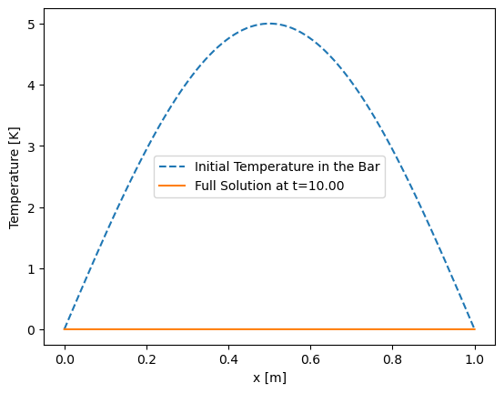
Let’s go ahead and plot this solution for \(\alpha=0.1\)m\(^2\)/s, L=1m. Before we start, let’s double check some units. \(\lambda_n\) should have units of 1/time $\(\lambda_n=\alpha\left(\frac{n\pi}{L}\right)^2=\left[\frac{m^2}{s}\right]\left(\frac{1}{[m]}\right)^2=\left[\frac{1}{s}\right]\)$

import numpy as np
import matplotlib.pyplot as plt

L=1 #m
alpha = 0.1 #m^2/s
lambdan = alpha*(np.pi/L)**2

x = np.linspace(0,L,100)

T0 = 5*np.sin(np.pi*x/L)
plt.plot(x,T0, '--', label='Initial Temperature in the Bar')
plt.xlabel('x [m]')
plt.ylabel('Temperature [K]')
plt.legend()

t = 10  #s
T = 5*np.exp(-lambdan*t)*np.sin(np.pi*x/L)

plt.plot(x, T, label='Full Solution at t=%1.2f'%t)
plt.legend()

<matplotlib.legend.Legend at 0x7f3d72856e60>

Really, we’re solving for the dynamics here, so let’s make this a little movie

import numpy as np
import matplotlib.pyplot as plt

from matplotlib import animation, rc
from IPython.display import HTML

# First set up the figure, the axis, and the plot element we want to animate
fig, ax = plt.subplots()
plt.close()

ax.plot(x,T0,'--',label='Initial Temp Profile')

ax.set_xlim(( -0.5, 1.5))
ax.set_ylim((0, 5))
ax.set_xlabel('x')
ax.set_ylabel('Temperature [K]')
line, = ax.plot([], [], lw=2, label='Temperature Profile')
ax.legend()

# initialization function: plot the background of each frame
def init():
    line.set_data([], [])
    return (line,)

# animation function. This is called sequentially  
def animate(i):

  T = 5*np.exp(-lambdan*t[i])*np.sin(np.pi*x/L)
  line.set_data(x, T)
  return (line,)
  
t = np.linspace(0,3,100)

anim = animation.FuncAnimation(fig, animate, init_func=init,
                             frames=100, interval=100, blit=True)

# Note: below is the part which makes it work on Colab
rc('animation', html='jshtml')
anim
  

Once Loop Reflect

This solution is saying that if we have a warm bar with a sin profile, and we hold it on both ends, the temperature will decay gradually like a sin.

More realistic boundary conditions

Solving a problem with a bar that has a sin temperature profile is not very interesting. How would you make a bar like that? I have no idea.

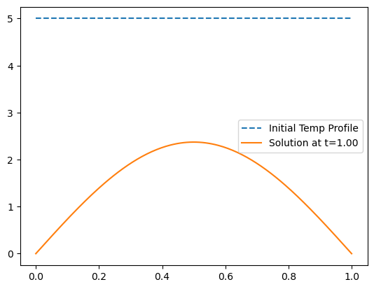
Let’s do a more reasonable set of initial conditions \(f(x)=5\), that is, we immerse the bar in a water bath 5 K warmer than our hands, then take it out and hold it out on both sides. We don’t have time to show how to solve this equation right now (we’ll do that next class). The magic \(c_n\) that specify this are

\[\begin{align*} c_n&= \begin{cases} \frac{4T_0}{n\pi} & n\text{ odd} \\ 0 & n\text{ even} \end{cases} \end{align*}\]

That makes our final solution

\[\begin{align*} T(x,t)&=\sum_{n=1}^{\infty} c_ne^{-\lambda_n t} \sin\left(\frac{n\pi x}{L}\right)\\ T(x,t)&=\sum_{n=1}^{\infty} \frac{20L}{n\pi}e^{-\lambda_n t} \sin\left(\frac{n\pi x}{L}\right) \end{align*}\]

import numpy as np
import matplotlib.pyplot as plt

L=1 #m
alpha=0.1 #m^2/s
T0 = 5

x = np.linspace(0, L, 200)

plt.plot(x,T0*np.ones(x.shape),'--',label='Initial Temp Profile')

t = 1 #initial profile
T = np.zeros(len(x))
for n in range(1,5):
  if n%2==1:
    cn=4*T0/np.pi/n
  else:
    cn=0
  lambdan=alpha*(n*np.pi/L)**2
  T=T+cn*np.exp(-lambdan*t)*np.sin(np.pi*n*x/L)

plt.plot(x,T,label='Solution at t=%1.2f'%t)
plt.legend()
ax.set_xlabel('x')
ax.set_ylabel('Temperature [K]')

Text(55.847222222222214, 0.5, 'Temperature [K]')

import numpy as np
import matplotlib.pyplot as plt

from matplotlib import animation, rc
from IPython.display import HTML


L=1 #m
alpha=0.1 #m^2/s
lambdan=alpha*(np.pi/L)**2
T0 = 5

x = np.linspace(0, L, 200)

# First set up the figure, the axis, and the plot element we want to animate
fig, ax = plt.subplots()
plt.close()

T0 = 5*np.ones(x.shape)
ax.plot(x,T0,'--',label='Initial Temp Profile')

ax.set_xlim(( -0.5, 1.5))
ax.set_ylim((0, 6))
ax.set_xlabel('x')
ax.set_ylabel('Temperature [K]')
line, = ax.plot([], [], lw=2, label='Temperature Profile')
ax.legend()

# initialization function: plot the background of each frame
def init():
    line.set_data([], [])
    return (line,)

# animation function. This is called sequentially  
def animate(i):
  T = np.zeros(len(x))
  for n in range(1,200):
    if n%2==1:
      cn=4*T0/np.pi/n
    else:
      cn=0
    lambdan=alpha*(n*np.pi/L)**2
    T=T+cn*np.exp(-lambdan*t[i])*np.sin(np.pi*n*x/L)
    
  line.set_data(x, T)
  return (line,)
  
t = np.linspace(0,3,100)

anim = animation.FuncAnimation(fig, animate, init_func=init,
                             frames=100, interval=100, blit=True)

# Note: below is the part which makes it work on Colab
rc('animation', html='jshtml')
anim
  

Once Loop Reflect

These magic \(c_n\) are called the Fourier coefficients. We’ll talk more on Tuesday about what they mean!