Recap for coupled differential equations:
Coupled homogeneous 1st order ODEs:
\(\vec{y'} = \arr{A} \vec{y}\) where \(\vec{y}\) is a vector of unknown functions.
\(\vec{y} = [y_1, y_2, y_3, ... y_n]^T\) represents an \(n^{th}\) order system with \(n\times n \ \arr{A}\)
We assumed that \(\vec{x}e^{\lambda t}\) was a solution, then showed that it was.
We proved that the eigenvalues and eigenvectors of \(\arr{A}\) yield the solution
(403)\[\begin{align}
\vec{y} = c_1\vec{x}^{(1)}e^{\lambda_1t} + c_2\vec{x}^{(2)}e^{\lambda_2t} + ... + c_n\vec{x}^{(n)}e^{\lambda_n t}
\end{align}\]
Now let’s look at complex eigenvalues
\(\underline{\text{Ex}}\):
(404)\[\begin{align}
y_1' &= 2y_2\\
y_2' &= -2y_1\\
\begin{bmatrix}y_1' \\ y_2' \end{bmatrix} &= \begin{bmatrix} 0 & 2 \\ -2 & 0 \end{bmatrix} \begin{bmatrix} y_1 \\ y_2 \end{bmatrix}\\
\implies \vec{y}' &= \arr{A}\vec{y} \text{ where } \arr{A} = \begin{bmatrix} 0 & 2 \\ -2 & 0 \end{bmatrix}
\end{align}\]
Can you guess what the solutions are going to look like?
Find eigenvalues of \(\arr{A}\):
(405)\[\begin{align}
\det(\arr{A} - \lambda\arr{I}) = 0\\
\left| \begin{array}{}0 - \lambda & 2 \\ -2 & 0-\lambda \end{array}\right| = 0 = \lambda^2 + 4\\
\lambda = \pm 2i \rightarrow \lambda_1 = 2i, \ \lambda_2 = -2i
\end{align}\]
Find eigenvectors
Set \((\arr{A} - \lambda\arr{I})\vec{x}^{(1)} = \vec{0}\)
(406)\[\begin{align}
\begin{bmatrix} -2i & 2 \\ -2 & -2i\end{bmatrix} \begin{bmatrix} x_1 \\ x_2 \end{bmatrix} = \begin{bmatrix} 0 \\ 0 \end{bmatrix}\\
\implies -2ix_1 + 2x_2 = 0\\
[-2x_1 - 2ix_2 = 0]i && \text{(redundant)}
\rightarrow -2ix_1 + 2x_2 = 0\\
ix_1 = x_2 \implies \vec{x}^{(1)} = \begin{bmatrix} 1 \\ i \end{bmatrix}
\end{align}\]
(407)\[\begin{align}
\begin{bmatrix} 2i & 2 \\ -2 & 2i \end{bmatrix} \begin{bmatrix} x_1 \\ x_2 \end{bmatrix} = \begin{bmatrix} 0 \\ 0 \end{bmatrix}\\
\implies 2ix_1 + 2x_2 = 0\\
-ix_1 = x_2 \implies \vec{x}^{(2)} = \begin{bmatrix} 1 \\ i \end{bmatrix} = \begin{bmatrix} i \\ 1 \end{bmatrix}
\end{align}\]
\(\therefore\) General solution is:
(408)\[\begin{align}
\vec{y} = c_1 \begin{bmatrix} 1 \\ i \end{bmatrix}e^{2it} + c_2 \begin{bmatrix} 1 \\ -i \end{bmatrix} e^{-2it}
\end{align}\]
Not very useful since it’s imaginary
(409)\[\begin{align}
e^{2it} &= \cos(2t) + i\sin(2t)\\
e^{-2it} &= \cos(-2t) + i\sin(-2t)\\
&= \cos(2t) - i\sin(2t)
\end{align}\]
(410)\[\begin{align}
\begin{bmatrix} 1 \\ i \end{bmatrix} e^{2it} &= \begin{bmatrix} 1 \\ i \end{bmatrix} (\cos 2t + i\sin 2t)\\
&= \begin{bmatrix} \cos 2t + i\sin 2t \\ i\cos 2t - \sin 2t \end{bmatrix}\\
&= \begin{bmatrix} \cos 2t \\ -\sin 2t \end{bmatrix} + i \begin{bmatrix} \sin 2t \\ \cos 2t\end{bmatrix}\\
&= \vec{a} + i\vec{b}\\
\begin{bmatrix} 1 \\ -i \end{bmatrix} e^{-2it} &= \begin{bmatrix} 1 \\ -i \end{bmatrix} (\cos 2t - i\sin 2t)\\
&= \begin{bmatrix} \cos 2t - i\sin 2t \\ -i\cos 2t - \sin 2t \end{bmatrix}\\
&= \begin{bmatrix} \cos 2t \\ -\sin 2t \end{bmatrix} - i \begin{bmatrix} \sin 2t \\ \cos 2t\end{bmatrix}\\
&= \vec{a} - i\vec{b}
\end{align}\]
(411)\[\begin{align}
\frac{1}{2} \left\{\begin{bmatrix} 1 \\ i \end{bmatrix} e^{2it} + \begin{bmatrix} 1 \\ -i\end{bmatrix}e^{-2it} \right\} &= \frac{1}{2}(\vec{a} + i\vec{b} + \vec{a} - i\vec{b})\\
&= \frac{1}{2}(2\vec{a})\\
&= \vec{a} && \rightarrow\text{the sum of two linearly independent solutions is also a solution}\\
-\frac{i}{2} \left\{\begin{bmatrix} 1 \\ i \end{bmatrix} e^{2it} - \begin{bmatrix} 1 \\ -i\end{bmatrix}e^{-2it} \right\} &= -\frac{i}{2}(\vec{a} + i\vec{b} - \vec{a} + i\vec{b})\\
&= -\frac{i}{2}\cdot 2i\vec{b}\\
&= \vec{b} && \rightarrow\text{the difference of two linearly independent solutions is also a solution}
\end{align}\]
\(\therefore \vec{y} = c_1 \vec{a} + c_2 \vec{b}\) is a real representation of the general solution
(412)\[\begin{align}
\vec{y} = c_1 \begin{bmatrix} \cos 2t \\ -\sin 2t \end{bmatrix} + c_2 \begin{bmatrix} \sin 2t \\ \cos 2t \end{bmatrix}
\end{align}\]
OR
(413)\[\begin{align}
y_1(t) &= c_1 \cos 2t + c_2 \sin 2t\\
y_2(t) &= -c_1\sin 2t + c_2\cos 2t
\end{align}\]
General solution for complex eigenvalues
We don’t have to go through all of this work every time!
(414)\[\begin{align}
\vec{y}=e^\lambda t\left[c_1(\vec{a}\cos\omega t-\vec{b}\sin \omega t)+c_2(\vec{a}\sin\omega t+\vec{b}\cos \omega t)\right]
\end{align}\]
To be clear, here \(\vec{a}\) is the real part of the eigenvector, and \(\vec{b}\) is the imaginary part of the eigenvector.
For the above example (\(\lambda=\pm 2i\), eigenvector \(\vec{x}=[1,\pm i]\), this yields
(415)\[\begin{align}
\vec{y}&=e^0 t\left[c_1\left(\begin{bmatrix}1\\0\end{bmatrix}\cos2 t-\begin{bmatrix}0\\1\end{bmatrix}\sin 2 t\right)+c_2\left(\begin{bmatrix}1\\0\end{bmatrix}\sin2 t+\begin{bmatrix}0\\1\end{bmatrix}\cos 2 t\right)\right]\\
y_1&=c_1\cos2t +c_2 \sin2t\\
y_2&=-c_1\sin 2t+c_2\cos2t
\end{align}\]
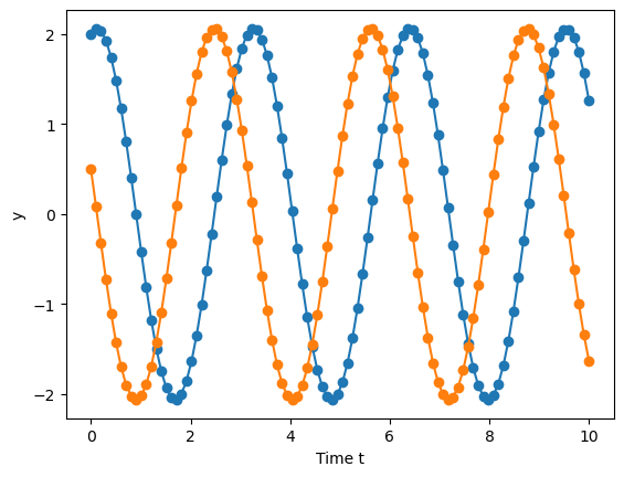
Numerical solution to this example
Remember, when we solve this numerically, we also need initial conditions. So let’s say that \(y_1(t=0)=2\) and \(y_2(t=0)=0.5\)
More than two coupled linear equations:
Very easy to add more to our systems
\(\underline{\text{Ex}}\):
(416)\[\begin{align}
y_1' &= 3y_1 + 5y_2 + 3y_3\\
y_2' &= 4y_2 + 6y_3\\
y_3' &= y_3
\end{align}\]
(417)\[\begin{align}
\vec{y}' = \arr{A}\vec{y} \ \text{ where } \vec{y} = \begin{bmatrix} y_1 \\ y_2 \\ y_3 \end{bmatrix} \text{ and } \arr{A} = \begin{bmatrix} 3 & 5 & 3 \\ 0 & 4 & 6 \\ 0 & 0 & 1 \end{bmatrix}
\end{align}\]
(418)\[\begin{align}
\vec{y} = c_1 \vec{x}^{(1)}e^{\lambda_1 t} + c_2 \vec{x}^{(2)}e^{\lambda_2 t} + c_3 \vec{x}^{(3)}e^{\lambda_3 t}
\end{align}\]
where \(\lambda\)’s are the eigenvalues of \(\arr{A}\) and \(\vec{x}^{(i)}\)’s are the eigenvectors of \(\arr{A}\)
(419)\[\begin{align}
\arr{A} &= \begin{bmatrix} 3 & 5 & 3 \\ 0 & 4 & 6 \\ 0 & 0 & 1 \end{bmatrix} \\
\implies \lambda_1 &= 3,\ \vec{x}^{(1)} = \begin{bmatrix} 1 & 0 & 0 \end{bmatrix}^T\\
\lambda_2 &= 4,\ \vec{x}^{(2)} = \begin{bmatrix} 5 & 1 & 0 \end{bmatrix}^T\\
\lambda_3 &= 1,\ \vec{x}^{(3)} = \begin{bmatrix} 7 & -4 & 2 \end{bmatrix}^T
\end{align}\]
(420)\[\begin{align}
\therefore \vec{y} = c_1 \begin{bmatrix} 1 \\ 0 \\ 0 \end{bmatrix} e^{3t} + c_2 \begin{bmatrix} 5 \\ 1 \\ 0 \end{bmatrix} e^{4t} + c_3 \begin{bmatrix} 7 \\ -4 \\ 2 \end{bmatrix} e^{t}
\end{align}\]
OR:
(421)\[\begin{align}
y_1(t) &= c_1 e^{3t} + 5c_2e^{4t} + 7c_3e^t\\
y_2(t) &= c_2e^{4t} - 4c_3e^t\\
y_3(t) &= 2c_3e^t
\end{align}\]
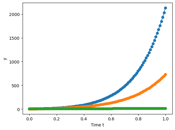
[3. 4. 1.]
[ 0.84270097 -0.48154341  0.24077171]
[ 7. -4.  2.]
Numerical solution
We need three initial conditions now. Let’s say \(y_1(0)=4, y_2(0)=2, y_3(0)=6\). Almost no changes from the above code
How do we handle non-homogeneous systems
\(\rightarrow\) Same idea as single equations
(422)\[\begin{align}
y_1' &= -3y_1 + y_2 + 3\cos t\\
y_2' &= y_1 -3y_2 -2\cos t -3\sin t\\
\begin{bmatrix} y_1' \\ y_2' \end{bmatrix} &= \begin{bmatrix} -3 & 1 \\ 1 & -3 \end{bmatrix} \begin{bmatrix} y_1 \\ y_2 \end{bmatrix} + \begin{bmatrix} 3\cos t \\ -2\cos t - 3\sin t \end{bmatrix}\\
\vec{y}' &= \arr{A}\vec{y} + \vec{g}(t) \text{ where $\vec{g}$ is a vector with no dependence on $\vec{y}$}
\end{align}\]
Solve homogeneous system. From \(\arr{A}\):
(423)\[\begin{align}
\lambda_1 = -4 && \vec{x}^{(1)} = \begin{bmatrix} -1 & 1 \end{bmatrix}^T\\
\lambda_2 = -2 && \vec{x}^{(2)} = \begin{bmatrix} 1 & 1 \end{bmatrix}^T
\end{align}\]
(424)\[\begin{align}
\therefore \vec{y}_H (t) = c_1\begin{bmatrix} -1 \\ 1 \end{bmatrix} e^{-4t} + c_2 \begin{bmatrix} 1 \\ 1 \end{bmatrix} e^{-2t}
\end{align}\]
Solve non-homogeneous part
Now, the particular solution \(\vec{y}_P\) is a vector
For this example use MoUC. Choose \(\vec{y}_P\) based on \(\vec{g} = \begin{bmatrix} 3\cos t \\ -2\cos t -3\sin t \end{bmatrix}\)
(425)\[\begin{align}
\vec{y}_P = \vec{u}\sin t + \vec{v}\cos t
\end{align}\]
where \(\vec{u} = \begin{bmatrix} u_1 \\ u_2 \end{bmatrix}\) and \(\vec{v} = \begin{bmatrix} v_1 \\ v_2 \end{bmatrix}\) are the vectors of undetermined coefficients.
Then, \(\vec{y}_P' = \vec{u} \cos t - \vec{v}\sin t\)
(426)\[\begin{align}
\vec{u}\cos t - \vec{v}\sin t = \arr{A}(\vec{u}\sin t + \vec{v}\cos t) + \vec{g}\\
(\vec{u} - \arr{A}\vec{v})\cos t - (\arr{A}\vec{u} + \vec{v})\sin t = \vec{g}
\end{align}\]
(427)\[\begin{align}
\vec{u} - \arr{A}\vec{v} = \begin{bmatrix} 3 \\ -2 \end{bmatrix}
\end{align}\]
* sin(t) terms (two equations):
\begin{align}
-\arr{A} \vec{u} -\vec{v} = \begin{bmatrix} 0 \\ -3 \end{bmatrix}
\end{align}
(428)\[\begin{align}
-\arr{A}\left(\begin{bmatrix} 3 \\ -2 \end{bmatrix} + \arr{A}\vec{v} \right) - \vec{v} = \begin{bmatrix} 0 \\ -3 \end{bmatrix}\\
\text{simplifies to }\ \begin{bmatrix} -11 & 6 \\ 6 & -11 \end{bmatrix} \begin{bmatrix}v_1 \\ v_2\end{bmatrix} = \begin{bmatrix} -11 \\ 6 \end{bmatrix}\\
\left[\begin{array}{ll|l}-11 & 6 & -11 \\ 6 & -11 & 6\end{array}\right] \text{ G.E} \rightarrow \left[\begin{array}{ll|l} 1&0&1 \\ 0&1&0\end{array} \right]\\
\therefore \vec{v} = \begin{bmatrix} 1 \\ 0 \end{bmatrix} \text{ and } \vec{u} = \begin{bmatrix} 3 \\ -2 \end{bmatrix} + \arr{A}\begin{bmatrix} 1 \\ 0 \end{bmatrix} = \begin{bmatrix} 0 \\ -1 \end{bmatrix}\\
\therefore \vec{y}_P = \begin{bmatrix} 0 \\ -1 \end{bmatrix} \sin t + \begin{bmatrix} 1 \\ 0 \end{bmatrix} \cos t
\end{align}\]
and
(429)\[\begin{align}
\vec{y}(t) = c_1 \begin{bmatrix} -1 \\ 1 \end{bmatrix} e^{-4t} + c_2 \begin{bmatrix} 1 \\ 1 \end{bmatrix} e^{-2t} + \begin{bmatrix} 0 \\ -1 \end{bmatrix} \sin t + \begin{bmatrix} 1 \\ 0 \end{bmatrix} \cos t
\end{align}\]
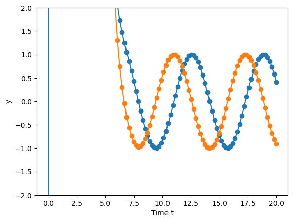
Notice that this says the initial conditions don’t matter after a while!!
Non-homogeneous system - VOP Method
(430)\[\begin{align}
y_1' &= -2y_1 + y_2 + 2e^{-t}\\
y_2' &= y_1 -2y_2 + 3t\\
\vec{y}' &= \arr{A}\vec{y} + \vec{g}(t)
\end{align}\]
Solve homogeneous system
from \(\arr{A} \rightarrow |\arr{A}-\lambda\arr{I}|=0\)
(431)\[\begin{align}
\left|\begin{array}{} -2-\lambda & 1 \\ 1 & -2-\lambda \end{array}\right| = 0 & = (-2-\lambda)(-2-\lambda) -1\\
&= +4 + 2\lambda + 2 \lambda + \lambda^2 - 1\\
&= \lambda^2 + 4\lambda + 3 = (\lambda + 3)(\lambda + 1)\\
\lambda_1 &= -3 ; \ \lambda_2 = -1
\end{align}\]
then \((\arr{A} - \lambda\arr{I})\vec{x} = \vec{0}\)
For \(\lambda_1=-3\)
(432)\[\begin{align}
\left[\begin{array}{ll|l} 1 & 1 & 0 \\ 1 & 1 & 0 \end{array} \right] \rightarrow x_1 + x_2 = 0 \implies x_1 = -x_2 \implies \vec{x}^{(1)} = \begin{bmatrix} 1 \\ -1 \end{bmatrix}
\end{align}\]
For \(\lambda_2=-1\)
(433)\[\begin{align}
\left[\begin{array}{ll|l} -1 & 1 & 0 \\ 1 & -1 & 0 \end{array} \right] \rightarrow -x_1 + x_2 = 0 \implies x_1 = x_2 \implies \vec{x}^{(2)} = \begin{bmatrix} 1 \\ 1 \end{bmatrix}
\end{align}\]
Then,
(434)\[\begin{align}
\vec{y}_H(t) = c_1 \begin{bmatrix} 1 \\ -1 \end{bmatrix} e^{-3t} + c_2\begin{bmatrix} 1 \\ 1 \end{bmatrix}e^{-t}
\end{align}\]
Solve non-homogeneous part using Variation of Parameters
(435)\[\begin{align}
\vec{y}_H(t) &= \begin{bmatrix} y_1^{(1)} & y_1^{(2)} \\ y_2^{(1)} & y_2^{(2)} \end{bmatrix} \begin{bmatrix} c_1 \\ c_2 \end{bmatrix} = \arr{Y}(t)\vec{c}\ \text{ where $\arr{Y}(t)$ is the $``$fundamental matrix"}\\
&= \begin{bmatrix} e^{-3t} & e^{-t} \\ -e^{-3t} & e^{-t}\end{bmatrix} \begin{bmatrix} c_1 \\ c_2 \end{bmatrix}
\end{align}\]
Just like with one dimensional case, we will form a particular solution by “replacing” the arbitrary constants of the homogeneous solution with an unknown function of \(t\), but this time with a vector. Assume \(\vec{y}_P(t) = \arr{Y}(t)\vec{u}(t)\)
We will determine \(\vec{u}(t)\) by substituting \(\vec{y}_P(t)\) into the original system
\(\rightarrow\) let’s derive in general terms
(436)\[\begin{align}
\vec{y}' &= \arr{A} \vec{y} + \vec{g} \\
\vec{y}_P' &= \arr{A}\vec{y}_P + \vec{g}\\
(\arr{Y}\vec{u})' &= \arr{A} \arr{Y}\vec{u} + \vec{g}\\
\arr{Y}'\vec{u} &+ \arr{Y}\vec{u}' = \arr{A}\arr{Y}\vec{u} + \vec{g}
\end{align}\]
\(\implies\) because \(\arr{Y}\) is a solution to the homogeneous system, we know it satifies \(\arr{Y}' = \arr{A}\arr{Y}\rightarrow\) substitute this in
(437)\[\begin{align}
\arr{A}\arr{Y}\vec{u} +\arr{Y}\vec{u}' &= \arr{A}\arr{Y}\vec{u} + \vec{g}\\
\arr{Y}^{-1}(\arr{Y}\vec{u}' &= \vec{g})
\end{align}\]
\(\rightarrow\) can multiply with inverse. We know \(\arr{Y}\) is non singular because \(\det(\arr{Y})=\) Wronskian which is non-zero for a basis
(438)\[\begin{align}
\vec{u}' &= \arr{Y}^{-1} \vec{g}\\
\vec{u}(t) &= \int \arr{Y}^{-1}(t) \vec{g}(t)dt + \vec{c} && \rightarrow \text{each element is integrated separately}
\end{align}\]
and
(439)\[\begin{align}
\vec{y}_P(t) &= \arr{Y}(t)\vec{u}(t)\\
&= \arr{Y}(t) \int \arr{Y}^{-1}(t)\vec{g}(t) dt
\end{align}\]
and
(440)\[\begin{align}
\vec{y}(t) &= \vec{y}_H + \vec{y}_P\\
\vec{y}(t) &= \arr{Y}(t)\vec{c} + \arr{Y}(t) \int \arr{Y}^{-1}(t)\vec{g}(t) dt
\end{align}\]
(441)\[\begin{align}
\arr{A}^{-1} = \frac{1}{\det \arr{A}}\begin{bmatrix} a_{22} & -a_{12} \\ -a_{21} & a_{11} \end{bmatrix}
\end{align}\]
then
(442)\[\begin{align}
\arr{Y}^{-1} &= \frac{1}{e^{-4t} + e^{-4t}} \begin{bmatrix} e^{-t} & -e^{-t} \\ e^{-3t} & e^{-3t} \end{bmatrix}\\
&=\frac{1}{2} \begin{bmatrix} e^{3t} & -e^{3t} \\ e^t & e^t \end{bmatrix}\\
\arr{Y}^{-1}\vec{g} &= \frac{1}{2}\begin{bmatrix} e^{3t} & -e^{3t} \\ e^t & e^t \end{bmatrix} \begin{bmatrix} 2e^{-t} \\ 3t\end{bmatrix} \\
&= \frac{1}{2} \begin{bmatrix} 2e^{2t} - 3te^{3t} \\ 2 + 3te^t \end{bmatrix}\\
\vec{u}(t) = \int \arr{Y}^{-1}\vec{g} &= \frac{1}{2} \begin{bmatrix} \int 2e^{2t}dt - \int 3te^{3t}dt \\ \int 2 dt + \int 3t e^t dt \end{bmatrix}\\
&=\frac{1}{2} \begin{bmatrix} e^{2t} - (te^{3t} - \frac{1}{3} e^{3t}) \\ 2t + 3(te^t - e^t) \end{bmatrix}
\end{align}\]
Then
(443)\[\begin{align}
\vec{y}_P(t) &= \arr{Y}(t)\vec{u}(t)\\
&= \begin{bmatrix} e^{-3t} & e^{-t} \\ -e^{-3t} & e^{-t} \end{bmatrix} \cdot \frac{1}{2} \cdot \begin{bmatrix} e^{2t}-te^{3t} + \frac{1}{3}e^{3t} \\ 2t + 3te^t - 3e^t \end{bmatrix} \\
&= \frac{1}{2} \begin{bmatrix} e^{-t} -t + \frac{1}{3} + 2te^{-t}+ 3t -3 \\ -e^{-t} + t -\frac{1}{3} + 2te^{-t} + 3t - 3 \end{bmatrix}\\
&= \begin{bmatrix} \frac{1}{2} e^{-t} + te^{-t} + t - \frac{4}{3} \\ -\frac{1}{2} e^{-t} + te^{-t} + 2t - \frac{5}{3}\end{bmatrix}\\
\vec{y}_P(t) &= \frac{1}{2}\begin{bmatrix} 1 \\ -1 \end{bmatrix} e^{-t} + \begin{bmatrix} 1 \\ 1\end{bmatrix} te^{-t} + \begin{bmatrix} 1 \\ 2 \end{bmatrix} t -\frac{1}{3}\begin{bmatrix} 4 \\ 5 \end{bmatrix}
\end{align}\]
Then,
(444)\[\begin{align}
\vec{y}(t) &= \vec{y}_H(t) + \vec{y}_P(t)\\
&= c_1 \begin{bmatrix} 1 \\ -1 \end{bmatrix} e^{-3t} + c_2 \begin{bmatrix} 1 \\ 1 \end{bmatrix} e^{-t} + \frac{1}{2}\begin{bmatrix} 1 \\ -1 \end{bmatrix} e^{-t} + \begin{bmatrix} 1 \\ 1 \end{bmatrix}te^{-t} + \begin{bmatrix} 1 \\ 2 \end{bmatrix} t - \frac{1}{3} \begin{bmatrix} 4 \\ 5 \end{bmatrix} && \text{general solution}
\end{align}\]
Numerical solution
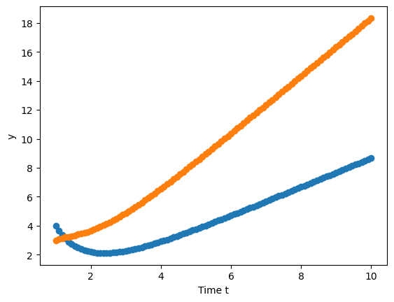
Integrate \(\vec{y}' = \begin{bmatrix}-2 & 1 \\ 1 & -2 \end{bmatrix}\vec{y} + \begin{bmatrix} 2e^{-t} \\ 3t \end{bmatrix}\), with the initial condition \(\vec{y}(t=1)=[4,3]^T\) from t=1 to t=10.