Non-linear regression
Contents
Non-linear regression#
Recap on linear regression#
Last class, we talked about how we could turn linear regression into a linear algebra problem
You can calculate this yourself
You can also do linear regression using statistical packages like statsmodel
Today we will discuss two ways of solving non-linear regression problems
Turn a non-linear problem into a linear one and solve
Non-linear curve fitting
Turn a non-linear regression problem into a linear regression problem#
Rate constants and reaction orders are determined by using models that are fit to experimental data
A common case is to monitor concentration vs. time in a constant volume, batch reactor
We consider the disappearance of \(A\)
From the mole balance we know:
Let us assume the rate law is of the form: \(r_A = k C_A^\alpha\) and a constant volume so that:
Let us be loose with mathematics, rearrange the equation, and take the log of both sides.
By loose I mean we take logs of quantities that are not dimensionless
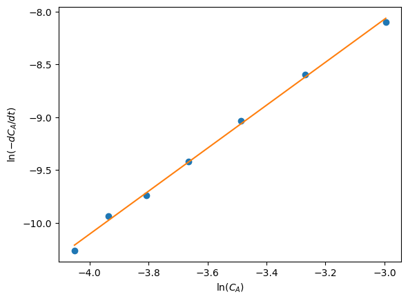
This suggests that if we could numerically compute \(\frac{dC_A}{dt}\) from our data of \(C_A(t)\) then a plot of the log of the negative derivative vs the log of concentration would have
an intercept equal to the log of the rate constant, \(k\)
and a slope equal to the reaction order \(\alpha\)
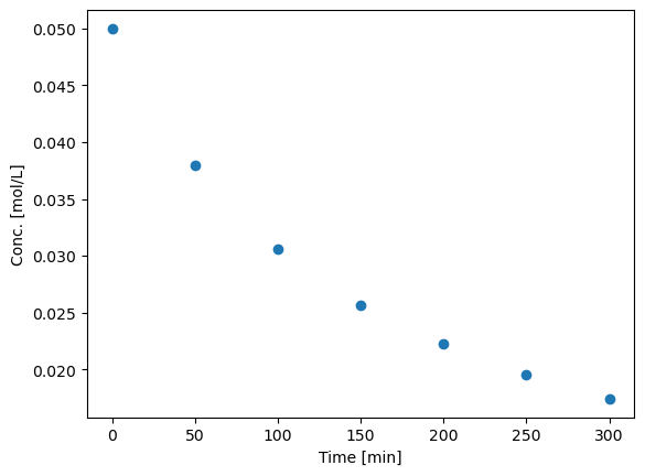
Given the following data, determine the reaction order in A and the rate constant with 95% confidence intervals.
| time (min) | C\_A (mol/L) |
|---|---|
| 0 | 0.0500 |
| 50 | 0.0380 |
| 100 | 0.0306 |
| 150 | 0.0256 |
| 200 | 0.0222 |
| 250 | 0.0195 |
| 300 | 0.0174 |
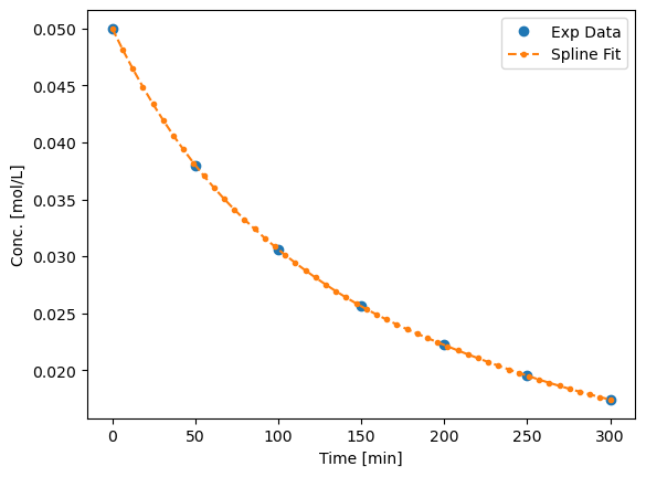
We can get the derivatives by first fitting a spline through the data. The spline is essentially just a smoothing function
We will use the
splevfunction to numerically compute derivatives from spline fits of the function.This works best when the \(x\) points are evenly spaced, and they should be monotically increasing or decreasing
import numpy as np
import matplotlib.pyplot as plt

data=np.array([[0,0.05],
               [50,.038],
               [100,.0306],
               [150,.0256],
               [200,.0222],
               [250,.0195],
               [300,.0174]])

plt.plot(data[:,0],data[:,1],'o')
plt.xlabel('Time [min]')
plt.ylabel('Conc. [mol/L]')
Text(0, 0.5, 'Conc. [mol/L]')
So, we need to convert the list of numbers to a numpy array so we can do the analysis.
import numpy as np
import matplotlib.pyplot as plt
from scipy import interpolate

# data will be a 2d list, which we convert to an array here
data = np.array(data)
t = data[:, 0]   # column 0
Ca = data[:, 1]  # column 1

# calculate a spline through the data
tck = interpolate.splrep(t, Ca)

t_eval = np.linspace(0,300)
Ca_spline = interpolate.splev(t_eval, tck)
plt.plot(data[:,0],data[:,1],'o', label='Exp Data')
plt.plot(t_eval, Ca_spline,'--.',label='Spline Fit')
plt.xlabel('Time [min]')
plt.ylabel('Conc. [mol/L]')
plt.legend()
<matplotlib.legend.Legend at 0x7f001ee04cd0>
import numpy as np
import matplotlib.pyplot as plt
from scipy import interpolate
import statsmodels.api as sm

# data will be a 2d list, which we convert to an array here
data = np.array(data)
t = data[:, 0]   # column 0
Ca = data[:, 1]  # column 1

# calculate numerical derivatives
tck = interpolate.splrep(t, Ca)
dCadt = interpolate.splev(t, tck, der=1)

# do the transformation
x = np.log(Ca)
y = np.log(-dCadt)

# setup and do the regression
# column of ones and x:  y = b + mx
X = np.column_stack([x, x**0])

mod = sm.OLS(y, X)
res = mod.fit()

intercept = res.params[1]
alpha = res.params[0]

confidence_intervals = res.conf_int(0.05)
intercept_error = confidence_intervals[1]
alpha_error = confidence_intervals[0]


print('alpha = {0}, conf interval {1}'.format(alpha, alpha_error))
print('k = {0}, conf interval {1}'.format(np.exp(intercept),
                                          np.exp(intercept_error)))


# always visually inspect the fit
plt.plot(x, y,'o')
plt.plot(x, res.predict(X))
plt.xlabel('$\ln(C_A)$')
plt.ylabel('$\ln(-dC_A/dt)$')
plt.show()
alpha = 2.0354816446001145, conf interval [1.92418422 2.14677907]
k = 0.1402128334966662, conf interval [0.09372748 0.20975319]
res.summary()
/home/runner/micromamba-root/envs/buildenv/lib/python3.10/site-packages/statsmodels/stats/stattools.py:74: ValueWarning: omni_normtest is not valid with less than 8 observations; 7 samples were given.
  warn("omni_normtest is not valid with less than 8 observations; %i "
| Dep. Variable: | y | R-squared: | 0.998 |
|---|---|---|---|
| Model: | OLS | Adj. R-squared: | 0.997 |
| Method: | Least Squares | F-statistic: | 2210. |
| Date: | Wed, 19 Oct 2022 | Prob (F-statistic): | 8.22e-08 |
| Time: | 19:29:39 | Log-Likelihood: | 13.785 |
| No. Observations: | 7 | AIC: | -23.57 |
| Df Residuals: | 5 | BIC: | -23.68 |
| Df Model: | 1 | ||
| Covariance Type: | nonrobust |
| coef | std err | t | P>|t| | [0.025 | 0.975] | |
|---|---|---|---|---|---|---|
| x1 | 2.0355 | 0.043 | 47.013 | 0.000 | 1.924 | 2.147 |
| const | -1.9646 | 0.157 | -12.539 | 0.000 | -2.367 | -1.562 |
| Omnibus: | nan | Durbin-Watson: | 2.377 |
|---|---|---|---|
| Prob(Omnibus): | nan | Jarque-Bera (JB): | 0.735 |
| Skew: | -0.181 | Prob(JB): | 0.692 |
| Kurtosis: | 1.454 | Cond. No. | 40.4 |
Notes:
[1] Standard Errors assume that the covariance matrix of the errors is correctly specified.
You can see there is a reasonably large range of values for the rate constant and reaction order (although the confidence interval does not contain zero)
The fit looks ok, but you can see the errors are not exactly random
There seems to be systematic trends in a sigmoidal shape of the data
That suggests small inadequacy in the model
Let us examine some methods of evaluating the quality of fit
First we examine the residuals, or the errors between the data and the model.
In a good fit, these will be randomly distributed
In a less good fit, there will be trends
residuals = y - res.predict(X)

# always visually inspect the fit
plt.plot(x, residuals, 'o-')
plt.xlabel('$\ln(C_A)$')
plt.ylabel('residuals')
plt.show()
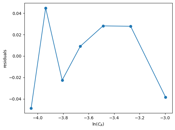
You can see there are trends in this data
That means the model may not be complete
There is uncertainty in the data
In each concentration measurement there is uncertainty in the time and value of concentration
You need more data to reduce the uncertainty
You may also need better data to reduce the uncertainty
Derivatives tend to magnify errors in data
The method we used to fit the data contributed to the uncertainty
We also nonlinearly transformed the errors by taking logs and exp of the data and results, which may have skewed the confidence limits
Nonlinear regression#
Nonlinear models are abundant in reaction engineering
\(r = k C_A^n \) is linear in the \(k\) parameter, and nonlinear in \(n\)
Nonlinear fitting is essentially a non-linear optimization problem
Unlike linear regression, where we directly compute the parameters using matrix algebra, we have to provide an initial guess and iterate to the solution
Similar to using fsolve, we must define a function of the model
The function takes an independent variable, and parameters, f(x,a,b,…)
The function should return a value of \(y\) for every value of \(x\)
i.e. it should be vectorized
It is possible to formulate these problems as nonlinear minimization of summed squared errors. See this example.
The function scipy.optimize.curve_fit provides nonlinear fitting of models (functions) to data.
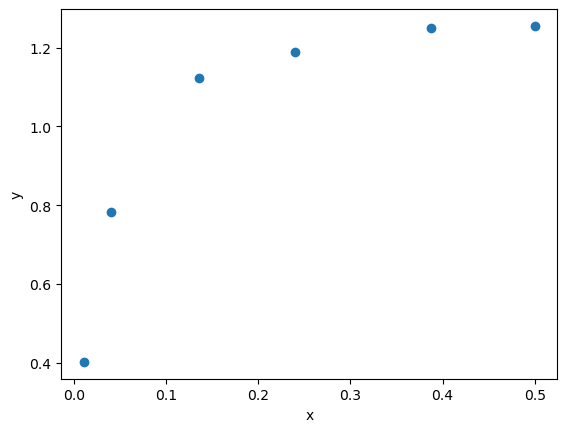
Let’s say we want to fit some other data to the function $\(y=ax/(b+x)\)$
import numpy as np

x = np.array([0.5, 0.387, 0.24, 0.136, 0.04, 0.011])
y = np.array([1.255, 1.25, 1.189, 1.124, 0.783, 0.402])


plt.plot(x,y,'o')
plt.xlabel('x')
plt.ylabel('y')
Text(0, 0.5, 'y')
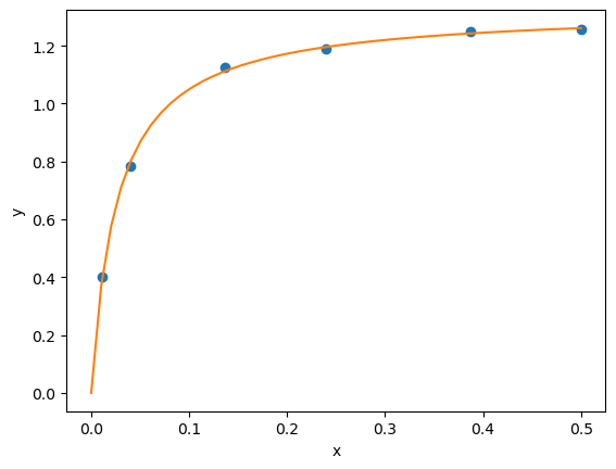
from scipy.optimize import curve_fit

def func(x, a, b):
    'nonlinear function in a and b to fit to data'
    return a * x / (b + x)

popt, pcov = curve_fit(func, x, y, p0=(3,3))


xrange = np.linspace(0,0.5)
fitted_y = func(xrange, *popt)

plt.plot(x,y,'o')
plt.plot(xrange,fitted_y)

plt.xlabel('x')
plt.ylabel('y')
Text(0, 0.5, 'y')

print(popt)
[1.32753142 0.02646156]
We also need to estimate uncertainties in nonlinear parameters
lmfitprovides a nice way to do this
Read the lmfit documentation to see how the confidence intervals are computed
Here is an example usage of lmfit.
!pip install lmfit
Requirement already satisfied: lmfit in /home/runner/micromamba-root/envs/buildenv/lib/python3.10/site-packages (1.0.3)
Requirement already satisfied: uncertainties>=3.0.1 in /home/runner/micromamba-root/envs/buildenv/lib/python3.10/site-packages (from lmfit) (3.1.7)
Requirement already satisfied: scipy>=1.4 in /home/runner/micromamba-root/envs/buildenv/lib/python3.10/site-packages (from lmfit) (1.9.2)
Requirement already satisfied: asteval>=0.9.22 in /home/runner/micromamba-root/envs/buildenv/lib/python3.10/site-packages (from lmfit) (0.9.27)
Requirement already satisfied: numpy>=1.18 in /home/runner/micromamba-root/envs/buildenv/lib/python3.10/site-packages (from lmfit) (1.23.4)
Requirement already satisfied: future in /home/runner/micromamba-root/envs/buildenv/lib/python3.10/site-packages (from uncertainties>=3.0.1->lmfit) (0.18.2)
from lmfit import Model

gmodel = Model(func, independent_vars=['x'],param_names=['a','b'])
params = gmodel.make_params(a=2., b=1.0)
result = gmodel.fit(y, params, x=x)

print(result.fit_report())
xrange = np.linspace(0,0.5)

fitted_y = result.eval(x=xrange)


plt.plot(x,y,'o')
plt.plot(xrange,fitted_y)

plt.xlabel('x')
plt.ylabel('y')
[[Model]]
    Model(func)
[[Fit Statistics]]
    # fitting method   = leastsq
    # function evals   = 36
    # data points      = 6
    # variables        = 2
    chi-square         = 6.9885e-04
    reduced chi-square = 1.7471e-04
    Akaike info crit   = -50.3470350
    Bayesian info crit = -50.7635160
[[Variables]]
    a:  1.32753139 +/- 0.00972276 (0.73%) (init = 2)
    b:  0.02646155 +/- 0.00102789 (3.88%) (init = 1)
[[Correlations]] (unreported correlations are < 0.100)
    C(a, b) = 0.711
Text(0, 0.5, 'y')
Here the two intervals are relatively small, and do not include zero, suggesting both parameters are significant.
More importantly, the errors are not skewed by a nonlinear transformation.
Note you have to provide an initial guess.
This will not always be easy to guess.
There may be more than one minimum in the fit also, so different guesses may give different parameters.